

20
J. F. Reis et al.
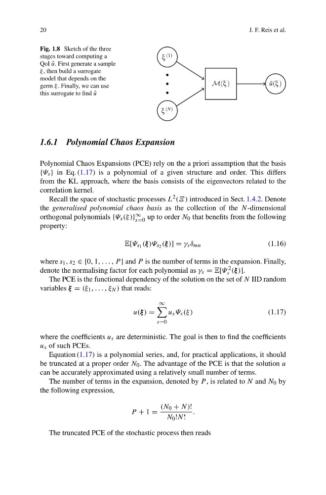
Fig. 1.8 Sketch of the three
stages toward computing a
QoI ˆ
u. First generate a sample
ξ , then build a surrogate
model that depends on the
germ ξ . Finally, we can use
this surrogate to find ˆ
u
M(ξ )
ξ (1)
ξ (N)
ˆ
u(ξ )
1.6.1 Polynomial Chaos Expansion
Polynomial Chaos Expansions (PCE) rely on the a priori assumption that the basis
{Ψ s } in Eq. (1.17) is a polynomial of a given structure and order. This differs
from the KL approach, where the basis consists of the eigenvectors related to the
correlation kernel.
Recall the space of stochastic processes L 2 (Ξ ) introduced in Sect. 1.4.2. Denote
the generalised polynomial chaos basis as the collection of the N -dimensional
orthogonal polynomials {Ψ s (ξ )} ∞
s=0 up to order N 0 that benefits from the following
property:
E[Ψ s 1 (ξ )Ψ s 2 (ξ )] = γ s δ mn
(1.16)
where s 1 , s 2 ∈ {0, 1, . . . , P } and P is the number of terms in the expansion. Finally,
denote the normalising factor for each polynomial as γ s = E[Ψ 2
s (ξ )].
The PCE is the functional dependency of the solution on the set of N IID random
variables ξ = (ξ 1 , . . . , ξ N ) that reads:
u(ξ ) =
∞
s=0
u s Ψ s (ξ )
(1.17)
where the coefficients u s are deterministic. The goal is then to find the coefficients
u s of such PCEs.
Equation (1.17) is a polynomial series, and, for practical applications, it should
be truncated at a proper order N 0 . The advantage of the PCE is that the solution u
can be accurately approximated using a relatively small number of terms.
The number of terms in the expansion, denoted by P , is related to N and N 0 by
the following expression,
P + 1 =
(N 0 + N)!
N 0 !N!
.
The truncated PCE of the stochastic process then reads
J. F. Reis et al.
Fig. 1.8 Sketch of the three
stages toward computing a
QoI ˆ
u. First generate a sample
ξ , then build a surrogate
model that depends on the
germ ξ . Finally, we can use
this surrogate to find ˆ
u
M(ξ )
ξ (1)
ξ (N)
ˆ
u(ξ )
1.6.1 Polynomial Chaos Expansion
Polynomial Chaos Expansions (PCE) rely on the a priori assumption that the basis
{Ψ s } in Eq. (1.17) is a polynomial of a given structure and order. This differs
from the KL approach, where the basis consists of the eigenvectors related to the
correlation kernel.
Recall the space of stochastic processes L 2 (Ξ ) introduced in Sect. 1.4.2. Denote
the generalised polynomial chaos basis as the collection of the N -dimensional
orthogonal polynomials {Ψ s (ξ )} ∞
s=0 up to order N 0 that benefits from the following
property:
E[Ψ s 1 (ξ )Ψ s 2 (ξ )] = γ s δ mn
(1.16)
where s 1 , s 2 ∈ {0, 1, . . . , P } and P is the number of terms in the expansion. Finally,
denote the normalising factor for each polynomial as γ s = E[Ψ 2
s (ξ )].
The PCE is the functional dependency of the solution on the set of N IID random
variables ξ = (ξ 1 , . . . , ξ N ) that reads:
u(ξ ) =
∞
s=0
u s Ψ s (ξ )
(1.17)
where the coefficients u s are deterministic. The goal is then to find the coefficients
u s of such PCEs.
Equation (1.17) is a polynomial series, and, for practical applications, it should
be truncated at a proper order N 0 . The advantage of the PCE is that the solution u
can be accurately approximated using a relatively small number of terms.
The number of terms in the expansion, denoted by P , is related to N and N 0 by
the following expression,
P + 1 =
(N 0 + N)!
N 0 !N!
.
The truncated PCE of the stochastic process then reads