

246
A. Riccardi et al.
• Specification of constraints
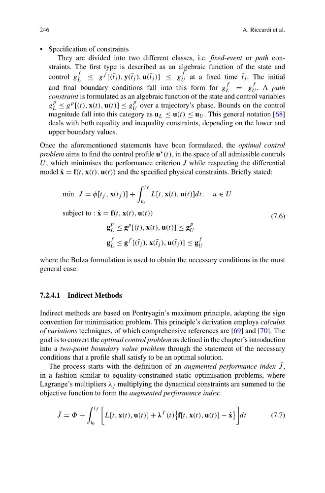
They are divided into two different classes, i.e. fixed-event or path constraints. The first type is described as an algebraic function of the state and
control g
f
L ≤ g f [(¯ t j ), y(¯ t j ), u(¯ t j )] ≤ g
f
U at a fixed time ¯
t j . The initial
and final boundary conditions fall into this form for g
f
L = g
f
U . A path
constraint is formulated as an algebraic function of the state and control variables
g
p
L ≤ g p [(t), x(t), u(t)] ≤ g
p
U over a trajectory’s phase. Bounds on the control
magnitude fall into this category as u L ≤ u(t) ≤ u U . This general notation [68]
deals with both equality and inequality constraints, depending on the lower and
upper boundary values.
Once the aforementioned statements have been formulated, the optimal control
problem aims to find the control profile u ∗ (t), in the space of all admissible controls
U , which minimises the performance criterion J while respecting the differential
model ˙
x = f(t, x(t), u(t)) and the specified physical constraints. Briefly stated:
min J = φ[t f , x(t f )] +
t f
t 0
L[t, x(t), u(t)]dt, u ∈ U
subject to : ˙
x = f(t, x(t), u(t))
g
p
L ≤ g
p
[(t), x(t), u(t)] ≤ g
p
U
g
f
L ≤ g
f
[(¯ t j ), x(¯ t j ), u(¯ t j )] ≤ g
f
U
(7.6)
where the Bolza formulation is used to obtain the necessary conditions in the most
general case.
7.2.4.1 Indirect Methods
Indirect methods are based on Pontryagin’s maximum principle, adapting the sign
convention for minimisation problem. This principle’s derivation employs calculus
of variations techniques, of which comprehensive references are [69] and [70]. The
goal is to convert the optimal control problem as defined in the chapter’s introduction
into a two-point boundary value problem through the statement of the necessary
conditions that a profile shall satisfy to be an optimal solution.
The process starts with the definition of an augmented performance index ¯
J ,
in a fashion similar to equality-constrained static optimisation problems, where
Lagrange’s multipliers λ j multiplying the dynamical constraints are summed to the
objective function to form the augmented performance index:
¯
J = Φ +
t f
t 0
L[t, x(t), u(t)] + λ
T (t)
f[t, x(t), u(t)] − ˙
x
dt
(7.7)
A. Riccardi et al.
• Specification of constraints
They are divided into two different classes, i.e. fixed-event or path constraints. The first type is described as an algebraic function of the state and
control g
f
L ≤ g f [(¯ t j ), y(¯ t j ), u(¯ t j )] ≤ g
f
U at a fixed time ¯
t j . The initial
and final boundary conditions fall into this form for g
f
L = g
f
U . A path
constraint is formulated as an algebraic function of the state and control variables
g
p
L ≤ g p [(t), x(t), u(t)] ≤ g
p
U over a trajectory’s phase. Bounds on the control
magnitude fall into this category as u L ≤ u(t) ≤ u U . This general notation [68]
deals with both equality and inequality constraints, depending on the lower and
upper boundary values.
Once the aforementioned statements have been formulated, the optimal control
problem aims to find the control profile u ∗ (t), in the space of all admissible controls
U , which minimises the performance criterion J while respecting the differential
model ˙
x = f(t, x(t), u(t)) and the specified physical constraints. Briefly stated:
min J = φ[t f , x(t f )] +
t f
t 0
L[t, x(t), u(t)]dt, u ∈ U
subject to : ˙
x = f(t, x(t), u(t))
g
p
L ≤ g
p
[(t), x(t), u(t)] ≤ g
p
U
g
f
L ≤ g
f
[(¯ t j ), x(¯ t j ), u(¯ t j )] ≤ g
f
U
(7.6)
where the Bolza formulation is used to obtain the necessary conditions in the most
general case.
7.2.4.1 Indirect Methods
Indirect methods are based on Pontryagin’s maximum principle, adapting the sign
convention for minimisation problem. This principle’s derivation employs calculus
of variations techniques, of which comprehensive references are [69] and [70]. The
goal is to convert the optimal control problem as defined in the chapter’s introduction
into a two-point boundary value problem through the statement of the necessary
conditions that a profile shall satisfy to be an optimal solution.
The process starts with the definition of an augmented performance index ¯
J ,
in a fashion similar to equality-constrained static optimisation problems, where
Lagrange’s multipliers λ j multiplying the dynamical constraints are summed to the
objective function to form the augmented performance index:
¯
J = Φ +
t f
t 0
L[t, x(t), u(t)] + λ
T (t)
f[t, x(t), u(t)] − ˙
x
dt
(7.7)