

7 Introduction to Optimisation
247
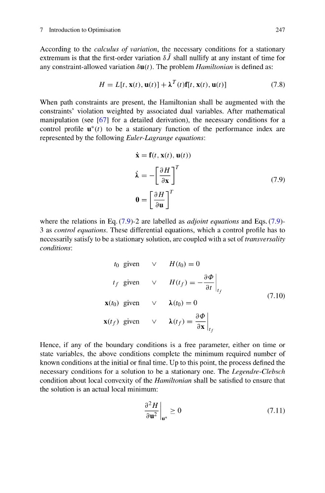
According to the calculus of variation, the necessary conditions for a stationary
extremum is that the first-order variation δ ¯
J shall nullify at any instant of time for
any constraint-allowed variation δu(t). The problem Hamiltonian is defined as:
H = L[t, x(t), u(t)] + λ
T (t)f[t, x(t), u(t)]
(7.8)
When path constraints are present, the Hamiltonian shall be augmented with the
constraints’ violation weighted by associated dual variables. After mathematical
manipulation (see [67] for a detailed derivation), the necessary conditions for a
control profile u ∗ (t) to be a stationary function of the performance index are
represented by the following Euler-Lagrange equations:
˙
x = f(t, x(t), u(t))
˙
λ = −
∂H
∂x
T
0 =
∂H
∂u
T
(7.9)
where the relations in Eq. (7.9)-2 are labelled as adjoint equations and Eqs. (7.9)3 as control equations. These differential equations, which a control profile has to
necessarily satisfy to be a stationary solution, are coupled with a set of transversality
conditions:
t 0 given
∨
H (t 0 ) = 0
t f given
∨
H (t f ) = −
∂Φ
∂t
t f
x(t 0 ) given
∨
λ(t 0 ) = 0
x(t f ) given
∨
λ(t f ) =
∂Φ
∂x
t f
(7.10)
Hence, if any of the boundary conditions is a free parameter, either on time or
state variables, the above conditions complete the minimum required number of
known conditions at the initial or final time. Up to this point, the process defined the
necessary conditions for a solution to be a stationary one. The Legendre-Clebsch
condition about local convexity of the Hamiltonian shall be satisfied to ensure that
the solution is an actual local minimum:
∂ 2 H
∂u 2
u ∗
≥ 0
(7.11)
247
According to the calculus of variation, the necessary conditions for a stationary
extremum is that the first-order variation δ ¯
J shall nullify at any instant of time for
any constraint-allowed variation δu(t). The problem Hamiltonian is defined as:
H = L[t, x(t), u(t)] + λ
T (t)f[t, x(t), u(t)]
(7.8)
When path constraints are present, the Hamiltonian shall be augmented with the
constraints’ violation weighted by associated dual variables. After mathematical
manipulation (see [67] for a detailed derivation), the necessary conditions for a
control profile u ∗ (t) to be a stationary function of the performance index are
represented by the following Euler-Lagrange equations:
˙
x = f(t, x(t), u(t))
˙
λ = −
∂H
∂x
T
0 =
∂H
∂u
T
(7.9)
where the relations in Eq. (7.9)-2 are labelled as adjoint equations and Eqs. (7.9)3 as control equations. These differential equations, which a control profile has to
necessarily satisfy to be a stationary solution, are coupled with a set of transversality
conditions:
t 0 given
∨
H (t 0 ) = 0
t f given
∨
H (t f ) = −
∂Φ
∂t
t f
x(t 0 ) given
∨
λ(t 0 ) = 0
x(t f ) given
∨
λ(t f ) =
∂Φ
∂x
t f
(7.10)
Hence, if any of the boundary conditions is a free parameter, either on time or
state variables, the above conditions complete the minimum required number of
known conditions at the initial or final time. Up to this point, the process defined the
necessary conditions for a solution to be a stationary one. The Legendre-Clebsch
condition about local convexity of the Hamiltonian shall be satisfied to ensure that
the solution is an actual local minimum:
∂ 2 H
∂u 2
u ∗
≥ 0
(7.11)