

6 Fundamentals of Filtering
189
p(x k |y 1:k ) =
p(y k |x k ) · p(x k |y 1:k−1 )
p(y k |x k ) · p(x k |y 1:k−1 )dx k
.
(6.19)
It has been shown above that the first term in the integral is computed by using the
observation model and the associated error probability function.
However, a tool to propagate the conditional probability in the time interval
between successive measurements, i.e. from p(x k−1 |y 1:k−1 ) at t k−1 to p(x k |y 1:k−1 )
at t k , is still needed. To this end, the differential equations governing the conditional
probability evolution will now be introduced.
6.1.3.1 Conditional Probability Evolution Between Observations
The missing bit of information to compute the posterior distribution in Eq. (6.19)
is how to obtain the new prior p(x k |y 1:k−1 ). This distribution characterises how the
state at time t k is influenced by previous observations, from t k−1 backwards. For its
computation, we suppose that the previous step in the sequential filtering scheme
has been solved, and therefore the probability p(x k−1 |y 1:k−1 ) is known. The goal of
this section is to present tools for the propagation of this conditional density from
t k−1 to t k when no new observations are received:
p(x k−1 |y 1:k−1 ) → p(x k |y 1:k−1 ) .
(6.20)
In the framework of Markov processes generated by stochastic differential
equations like Eq. (6.1), Kolmogorov derived equations for the exact evolution of
the density function p(t, x), characterising the process state, and for the process
transition density p(t, x t |τ, x τ ), characterising the process state evolution. The
Kolmogorov forward equation, also known as Fokker-Planck or KolmogorovFokker-Planck, is a partial differential equation that, for Markov diffusion processes,
is given by Challa and Faruqi [13] and Risken [47]:
∂p
∂t
= −
i
∂pf i
∂x i
+
1
2
i
j
∂ 2 p
GQG T
ij
∂x i ∂x j
,
(6.21)
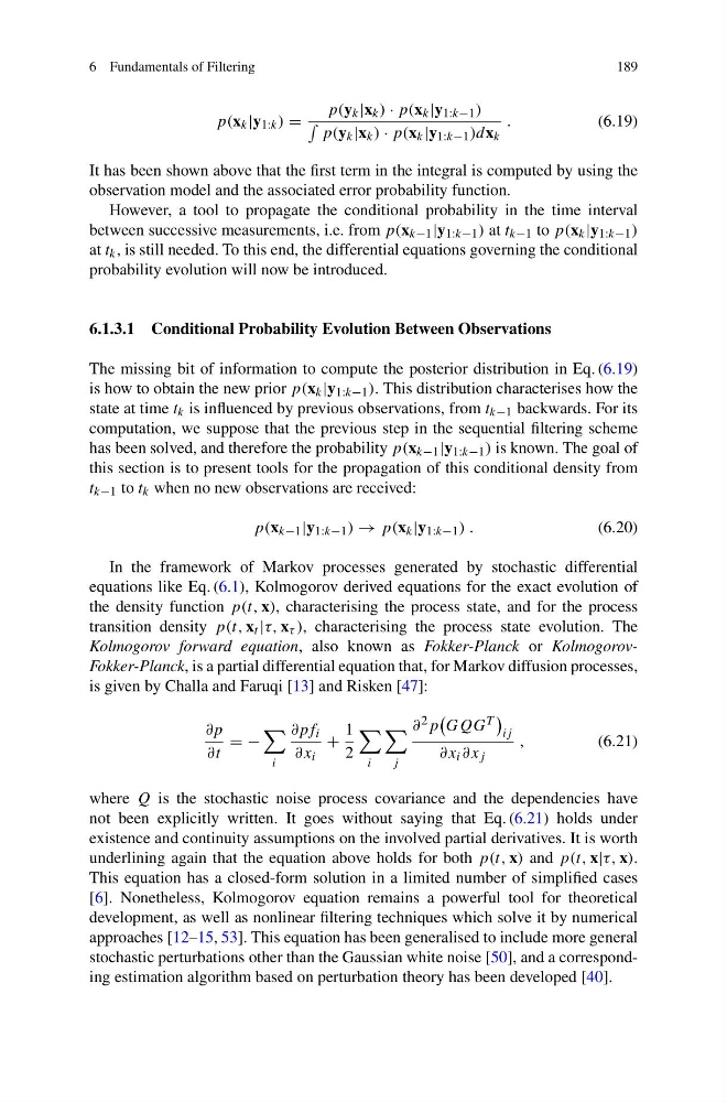
where Q is the stochastic noise process covariance and the dependencies have
not been explicitly written. It goes without saying that Eq. (6.21) holds under
existence and continuity assumptions on the involved partial derivatives. It is worth
underlining again that the equation above holds for both p(t, x) and p(t, x|τ, x).
This equation has a closed-form solution in a limited number of simplified cases
[6]. Nonetheless, Kolmogorov equation remains a powerful tool for theoretical
development, as well as nonlinear filtering techniques which solve it by numerical
approaches [12–15, 53]. This equation has been generalised to include more general
stochastic perturbations other than the Gaussian white noise [50], and a corresponding estimation algorithm based on perturbation theory has been developed [40].
189
p(x k |y 1:k ) =
p(y k |x k ) · p(x k |y 1:k−1 )
p(y k |x k ) · p(x k |y 1:k−1 )dx k
.
(6.19)
It has been shown above that the first term in the integral is computed by using the
observation model and the associated error probability function.
However, a tool to propagate the conditional probability in the time interval
between successive measurements, i.e. from p(x k−1 |y 1:k−1 ) at t k−1 to p(x k |y 1:k−1 )
at t k , is still needed. To this end, the differential equations governing the conditional
probability evolution will now be introduced.
6.1.3.1 Conditional Probability Evolution Between Observations
The missing bit of information to compute the posterior distribution in Eq. (6.19)
is how to obtain the new prior p(x k |y 1:k−1 ). This distribution characterises how the
state at time t k is influenced by previous observations, from t k−1 backwards. For its
computation, we suppose that the previous step in the sequential filtering scheme
has been solved, and therefore the probability p(x k−1 |y 1:k−1 ) is known. The goal of
this section is to present tools for the propagation of this conditional density from
t k−1 to t k when no new observations are received:
p(x k−1 |y 1:k−1 ) → p(x k |y 1:k−1 ) .
(6.20)
In the framework of Markov processes generated by stochastic differential
equations like Eq. (6.1), Kolmogorov derived equations for the exact evolution of
the density function p(t, x), characterising the process state, and for the process
transition density p(t, x t |τ, x τ ), characterising the process state evolution. The
Kolmogorov forward equation, also known as Fokker-Planck or KolmogorovFokker-Planck, is a partial differential equation that, for Markov diffusion processes,
is given by Challa and Faruqi [13] and Risken [47]:
∂p
∂t
= −
i
∂pf i
∂x i
+
1
2
i
j
∂ 2 p
GQG T
ij
∂x i ∂x j
,
(6.21)
where Q is the stochastic noise process covariance and the dependencies have
not been explicitly written. It goes without saying that Eq. (6.21) holds under
existence and continuity assumptions on the involved partial derivatives. It is worth
underlining again that the equation above holds for both p(t, x) and p(t, x|τ, x).
This equation has a closed-form solution in a limited number of simplified cases
[6]. Nonetheless, Kolmogorov equation remains a powerful tool for theoretical
development, as well as nonlinear filtering techniques which solve it by numerical
approaches [12–15, 53]. This equation has been generalised to include more general
stochastic perturbations other than the Gaussian white noise [50], and a corresponding estimation algorithm based on perturbation theory has been developed [40].