

190
C. Greco and M. Vasile
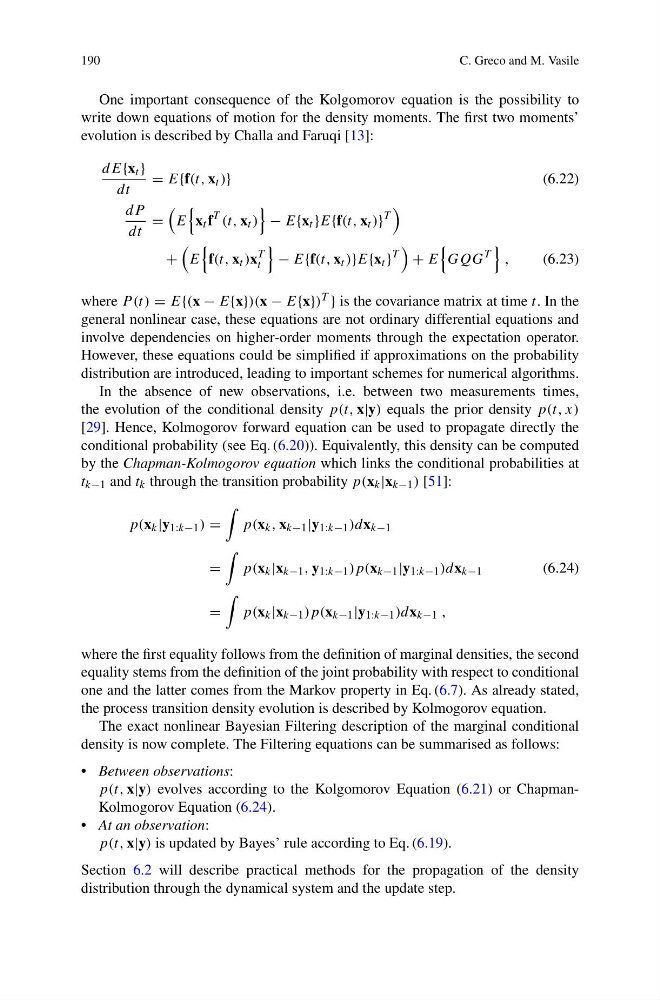
One important consequence of the Kolgomorov equation is the possibility to
write down equations of motion for the density moments. The first two moments’
evolution is described by Challa and Faruqi [13]:
dE{x t }
dt
= E{f(t, x t )}
(6.22)
dP
dt
=
E
x t f
T (t, x t )
− E{x t }E{f(t, x t )}
T
+
E
f(t, x t )x
T
t
− E{f(t, x t )}E{x t }
T
+ E
GQG
T
,
(6.23)
where P (t) = E{(x − E{x})(x − E{x}) T } is the covariance matrix at time t. In the
general nonlinear case, these equations are not ordinary differential equations and
involve dependencies on higher-order moments through the expectation operator.
However, these equations could be simplified if approximations on the probability
distribution are introduced, leading to important schemes for numerical algorithms.
In the absence of new observations, i.e. between two measurements times,
the evolution of the conditional density p(t, x|y) equals the prior density p(t, x)
[29]. Hence, Kolmogorov forward equation can be used to propagate directly the
conditional probability (see Eq. (6.20)). Equivalently, this density can be computed
by the Chapman-Kolmogorov equation which links the conditional probabilities at
t k−1 and t k through the transition probability p(x k |x k−1 ) [51]:
p(x k |y 1:k−1 ) =
p(x k , x k−1 |y 1:k−1 )dx k−1
=
p(x k |x k−1 , y 1:k−1 )p(x k−1 |y 1:k−1 )dx k−1
=
p(x k |x k−1 )p(x k−1 |y 1:k−1 )dx k−1 ,
(6.24)
where the first equality follows from the definition of marginal densities, the second
equality stems from the definition of the joint probability with respect to conditional
one and the latter comes from the Markov property in Eq. (6.7). As already stated,
the process transition density evolution is described by Kolmogorov equation.
The exact nonlinear Bayesian Filtering description of the marginal conditional
density is now complete. The Filtering equations can be summarised as follows:
• Between observations:
p(t, x|y) evolves according to the Kolgomorov Equation (6.21) or ChapmanKolmogorov Equation (6.24).
• At an observation:
p(t, x|y) is updated by Bayes’ rule according to Eq. (6.19).
Section 6.2 will describe practical methods for the propagation of the density
distribution through the dynamical system and the update step.
C. Greco and M. Vasile
One important consequence of the Kolgomorov equation is the possibility to
write down equations of motion for the density moments. The first two moments’
evolution is described by Challa and Faruqi [13]:
dE{x t }
dt
= E{f(t, x t )}
(6.22)
dP
dt
=
E
x t f
T (t, x t )
− E{x t }E{f(t, x t )}
T
+
E
f(t, x t )x
T
t
− E{f(t, x t )}E{x t }
T
+ E
GQG
T
,
(6.23)
where P (t) = E{(x − E{x})(x − E{x}) T } is the covariance matrix at time t. In the
general nonlinear case, these equations are not ordinary differential equations and
involve dependencies on higher-order moments through the expectation operator.
However, these equations could be simplified if approximations on the probability
distribution are introduced, leading to important schemes for numerical algorithms.
In the absence of new observations, i.e. between two measurements times,
the evolution of the conditional density p(t, x|y) equals the prior density p(t, x)
[29]. Hence, Kolmogorov forward equation can be used to propagate directly the
conditional probability (see Eq. (6.20)). Equivalently, this density can be computed
by the Chapman-Kolmogorov equation which links the conditional probabilities at
t k−1 and t k through the transition probability p(x k |x k−1 ) [51]:
p(x k |y 1:k−1 ) =
p(x k , x k−1 |y 1:k−1 )dx k−1
=
p(x k |x k−1 , y 1:k−1 )p(x k−1 |y 1:k−1 )dx k−1
=
p(x k |x k−1 )p(x k−1 |y 1:k−1 )dx k−1 ,
(6.24)
where the first equality follows from the definition of marginal densities, the second
equality stems from the definition of the joint probability with respect to conditional
one and the latter comes from the Markov property in Eq. (6.7). As already stated,
the process transition density evolution is described by Kolmogorov equation.
The exact nonlinear Bayesian Filtering description of the marginal conditional
density is now complete. The Filtering equations can be summarised as follows:
• Between observations:
p(t, x|y) evolves according to the Kolgomorov Equation (6.21) or ChapmanKolmogorov Equation (6.24).
• At an observation:
p(t, x|y) is updated by Bayes’ rule according to Eq. (6.19).
Section 6.2 will describe practical methods for the propagation of the density
distribution through the dynamical system and the update step.