

188
C. Greco and M. Vasile
where the last identity stems from the conditional independence of the observations
again.
It is straightforward to see how the latter suits a sequential formulation, where
the prior p(x k |y 1:k−1 ) of the current step is computed by propagating the posterior
p(x k−1 |y 1:k−1 ) of the previous one
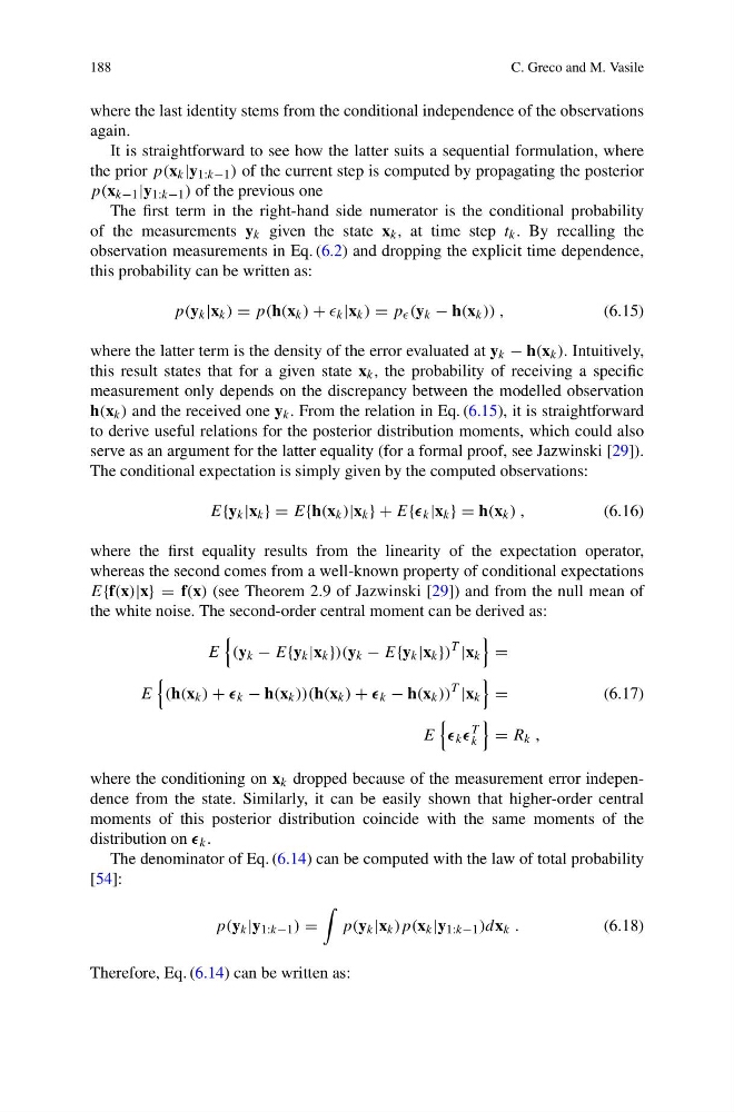
The first term in the right-hand side numerator is the conditional probability
of the measurements y k given the state x k , at time step t k . By recalling the
observation measurements in Eq. (6.2) and dropping the explicit time dependence,
this probability can be written as:
p(y k |x k ) = p(h(x k ) + k |x k ) = p (y k − h(x k )) ,
(6.15)
where the latter term is the density of the error evaluated at y k − h(x k ). Intuitively,
this result states that for a given state x k , the probability of receiving a specific
measurement only depends on the discrepancy between the modelled observation
h(x k ) and the received one y k . From the relation in Eq. (6.15), it is straightforward
to derive useful relations for the posterior distribution moments, which could also
serve as an argument for the latter equality (for a formal proof, see Jazwinski [29]).
The conditional expectation is simply given by the computed observations:
E{y k |x k } = E{h(x k )|x k } + E{ k |x k } = h(x k ) ,
(6.16)
where the first equality results from the linearity of the expectation operator,
whereas the second comes from a well-known property of conditional expectations
E{f(x)|x} = f(x) (see Theorem 2.9 of Jazwinski [29]) and from the null mean of
the white noise. The second-order central moment can be derived as:
E
(y k − E{y k |x k })(y k − E{y k |x k })
T
|x k
=
E
(h(x k ) + k − h(x k ))(h(x k ) + k − h(x k ))
T
|x k
=
E
k
T
k
= R k ,
(6.17)
where the conditioning on x k dropped because of the measurement error independence from the state. Similarly, it can be easily shown that higher-order central
moments of this posterior distribution coincide with the same moments of the
distribution on k .
The denominator of Eq. (6.14) can be computed with the law of total probability
[54]:
p(y k |y 1:k−1 ) =
p(y k |x k )p(x k |y 1:k−1 )dx k .
(6.18)
Therefore, Eq. (6.14) can be written as:
C. Greco and M. Vasile
where the last identity stems from the conditional independence of the observations
again.
It is straightforward to see how the latter suits a sequential formulation, where
the prior p(x k |y 1:k−1 ) of the current step is computed by propagating the posterior
p(x k−1 |y 1:k−1 ) of the previous one
The first term in the right-hand side numerator is the conditional probability
of the measurements y k given the state x k , at time step t k . By recalling the
observation measurements in Eq. (6.2) and dropping the explicit time dependence,
this probability can be written as:
p(y k |x k ) = p(h(x k ) + k |x k ) = p (y k − h(x k )) ,
(6.15)
where the latter term is the density of the error evaluated at y k − h(x k ). Intuitively,
this result states that for a given state x k , the probability of receiving a specific
measurement only depends on the discrepancy between the modelled observation
h(x k ) and the received one y k . From the relation in Eq. (6.15), it is straightforward
to derive useful relations for the posterior distribution moments, which could also
serve as an argument for the latter equality (for a formal proof, see Jazwinski [29]).
The conditional expectation is simply given by the computed observations:
E{y k |x k } = E{h(x k )|x k } + E{ k |x k } = h(x k ) ,
(6.16)
where the first equality results from the linearity of the expectation operator,
whereas the second comes from a well-known property of conditional expectations
E{f(x)|x} = f(x) (see Theorem 2.9 of Jazwinski [29]) and from the null mean of
the white noise. The second-order central moment can be derived as:
E
(y k − E{y k |x k })(y k − E{y k |x k })
T
|x k
=
E
(h(x k ) + k − h(x k ))(h(x k ) + k − h(x k ))
T
|x k
=
E
k
T
k
= R k ,
(6.17)
where the conditioning on x k dropped because of the measurement error independence from the state. Similarly, it can be easily shown that higher-order central
moments of this posterior distribution coincide with the same moments of the
distribution on k .
The denominator of Eq. (6.14) can be computed with the law of total probability
[54]:
p(y k |y 1:k−1 ) =
p(y k |x k )p(x k |y 1:k−1 )dx k .
(6.18)
Therefore, Eq. (6.14) can be written as: