

6 Fundamentals of Filtering
187
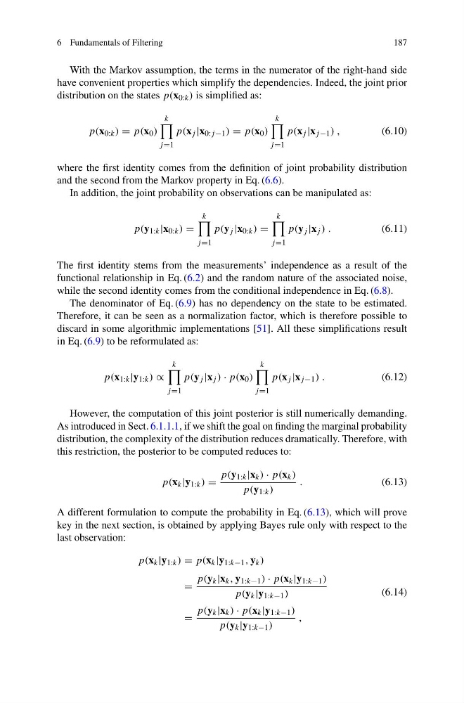
With the Markov assumption, the terms in the numerator of the right-hand side
have convenient properties which simplify the dependencies. Indeed, the joint prior
distribution on the states p(x 0:k ) is simplified as:
p(x 0:k ) = p(x 0 )
k
j =1
p(x j |x 0:j −1 ) = p(x 0 )
k
j =1
p(x j |x j −1 ) ,
(6.10)
where the first identity comes from the definition of joint probability distribution
and the second from the Markov property in Eq. (6.6).
In addition, the joint probability on observations can be manipulated as:
p(y 1:k |x 0:k ) =
k
j =1
p(y j |x 0:k ) =
k
j =1
p(y j |x j ) .
(6.11)
The first identity stems from the measurements’ independence as a result of the
functional relationship in Eq. (6.2) and the random nature of the associated noise,
while the second identity comes from the conditional independence in Eq. (6.8).
The denominator of Eq. (6.9) has no dependency on the state to be estimated.
Therefore, it can be seen as a normalization factor, which is therefore possible to
discard in some algorithmic implementations [51]. All these simplifications result
in Eq. (6.9) to be reformulated as:
p(x 1:k |y 1:k ) ∝
k
j =1
p(y j |x j ) · p(x 0 )
k
j =1
p(x j |x j −1 ) .
(6.12)
However, the computation of this joint posterior is still numerically demanding.
As introduced in Sect. 6.1.1.1, if we shift the goal on finding the marginal probability
distribution, the complexity of the distribution reduces dramatically. Therefore, with
this restriction, the posterior to be computed reduces to:
p(x k |y 1:k ) =
p(y 1:k |x k ) · p(x k )
p(y 1:k )
.
(6.13)
A different formulation to compute the probability in Eq. (6.13), which will prove
key in the next section, is obtained by applying Bayes rule only with respect to the
last observation:
p(x k |y 1:k ) = p(x k |y 1:k−1 , y k )
=
p(y k |x k , y 1:k−1 ) · p(x k |y 1:k−1 )
p(y k |y 1:k−1 )
=
p(y k |x k ) · p(x k |y 1:k−1 )
p(y k |y 1:k−1 )
,
(6.14)
187
With the Markov assumption, the terms in the numerator of the right-hand side
have convenient properties which simplify the dependencies. Indeed, the joint prior
distribution on the states p(x 0:k ) is simplified as:
p(x 0:k ) = p(x 0 )
k
j =1
p(x j |x 0:j −1 ) = p(x 0 )
k
j =1
p(x j |x j −1 ) ,
(6.10)
where the first identity comes from the definition of joint probability distribution
and the second from the Markov property in Eq. (6.6).
In addition, the joint probability on observations can be manipulated as:
p(y 1:k |x 0:k ) =
k
j =1
p(y j |x 0:k ) =
k
j =1
p(y j |x j ) .
(6.11)
The first identity stems from the measurements’ independence as a result of the
functional relationship in Eq. (6.2) and the random nature of the associated noise,
while the second identity comes from the conditional independence in Eq. (6.8).
The denominator of Eq. (6.9) has no dependency on the state to be estimated.
Therefore, it can be seen as a normalization factor, which is therefore possible to
discard in some algorithmic implementations [51]. All these simplifications result
in Eq. (6.9) to be reformulated as:
p(x 1:k |y 1:k ) ∝
k
j =1
p(y j |x j ) · p(x 0 )
k
j =1
p(x j |x j −1 ) .
(6.12)
However, the computation of this joint posterior is still numerically demanding.
As introduced in Sect. 6.1.1.1, if we shift the goal on finding the marginal probability
distribution, the complexity of the distribution reduces dramatically. Therefore, with
this restriction, the posterior to be computed reduces to:
p(x k |y 1:k ) =
p(y 1:k |x k ) · p(x k )
p(y 1:k )
.
(6.13)
A different formulation to compute the probability in Eq. (6.13), which will prove
key in the next section, is obtained by applying Bayes rule only with respect to the
last observation:
p(x k |y 1:k ) = p(x k |y 1:k−1 , y k )
=
p(y k |x k , y 1:k−1 ) · p(x k |y 1:k−1 )
p(y k |y 1:k−1 )
=
p(y k |x k ) · p(x k |y 1:k−1 )
p(y k |y 1:k−1 )
,
(6.14)