

186
C. Greco and M. Vasile
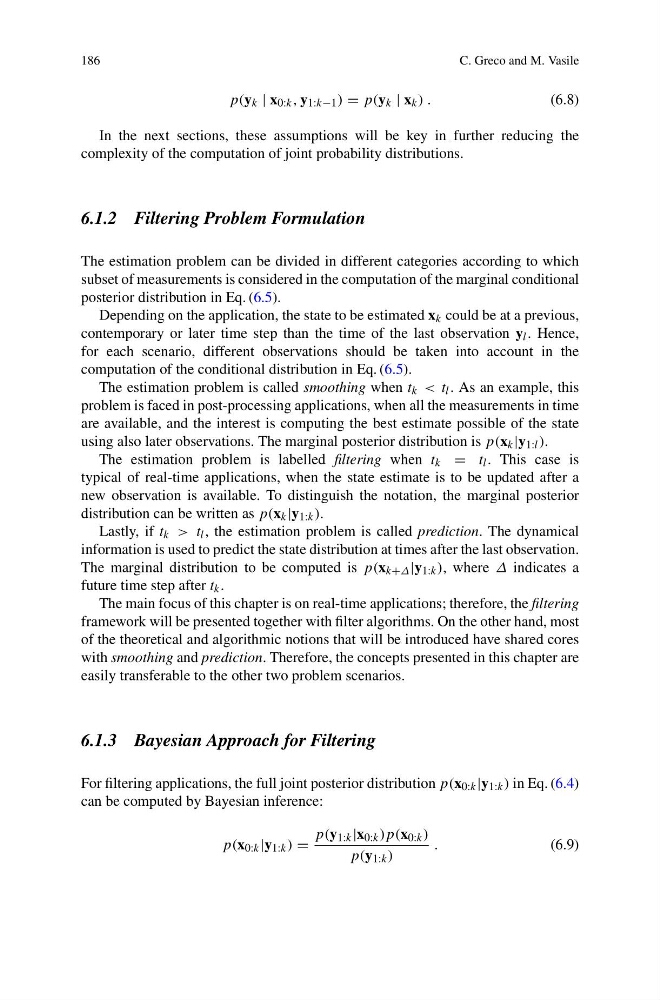
p(y k | x 0:k , y 1:k−1 ) = p(y k | x k ) .
(6.8)
In the next sections, these assumptions will be key in further reducing the
complexity of the computation of joint probability distributions.
6.1.2 Filtering Problem Formulation
The estimation problem can be divided in different categories according to which
subset of measurements is considered in the computation of the marginal conditional
posterior distribution in Eq. (6.5).
Depending on the application, the state to be estimated x k could be at a previous,
contemporary or later time step than the time of the last observation y l . Hence,
for each scenario, different observations should be taken into account in the
computation of the conditional distribution in Eq. (6.5).
The estimation problem is called smoothing when t k < t l . As an example, this
problem is faced in post-processing applications, when all the measurements in time
are available, and the interest is computing the best estimate possible of the state
using also later observations. The marginal posterior distribution is p(x k |y 1:l ).
The estimation problem is labelled filtering when t k = t l . This case is
typical of real-time applications, when the state estimate is to be updated after a
new observation is available. To distinguish the notation, the marginal posterior
distribution can be written as p(x k |y 1:k ).
Lastly, if t k > t l , the estimation problem is called prediction. The dynamical
information is used to predict the state distribution at times after the last observation.
The marginal distribution to be computed is p(x k+Δ |y 1:k ), where Δ indicates a
future time step after t k .
The main focus of this chapter is on real-time applications; therefore, the filtering
framework will be presented together with filter algorithms. On the other hand, most
of the theoretical and algorithmic notions that will be introduced have shared cores
with smoothing and prediction. Therefore, the concepts presented in this chapter are
easily transferable to the other two problem scenarios.
6.1.3 Bayesian Approach for Filtering
For filtering applications, the full joint posterior distribution p(x 0:k |y 1:k ) in Eq. (6.4)
can be computed by Bayesian inference:
p(x 0:k |y 1:k ) =
p(y 1:k |x 0:k )p(x 0:k )
p(y 1:k )
.
(6.9)
C. Greco and M. Vasile
p(y k | x 0:k , y 1:k−1 ) = p(y k | x k ) .
(6.8)
In the next sections, these assumptions will be key in further reducing the
complexity of the computation of joint probability distributions.
6.1.2 Filtering Problem Formulation
The estimation problem can be divided in different categories according to which
subset of measurements is considered in the computation of the marginal conditional
posterior distribution in Eq. (6.5).
Depending on the application, the state to be estimated x k could be at a previous,
contemporary or later time step than the time of the last observation y l . Hence,
for each scenario, different observations should be taken into account in the
computation of the conditional distribution in Eq. (6.5).
The estimation problem is called smoothing when t k < t l . As an example, this
problem is faced in post-processing applications, when all the measurements in time
are available, and the interest is computing the best estimate possible of the state
using also later observations. The marginal posterior distribution is p(x k |y 1:l ).
The estimation problem is labelled filtering when t k = t l . This case is
typical of real-time applications, when the state estimate is to be updated after a
new observation is available. To distinguish the notation, the marginal posterior
distribution can be written as p(x k |y 1:k ).
Lastly, if t k > t l , the estimation problem is called prediction. The dynamical
information is used to predict the state distribution at times after the last observation.
The marginal distribution to be computed is p(x k+Δ |y 1:k ), where Δ indicates a
future time step after t k .
The main focus of this chapter is on real-time applications; therefore, the filtering
framework will be presented together with filter algorithms. On the other hand, most
of the theoretical and algorithmic notions that will be introduced have shared cores
with smoothing and prediction. Therefore, the concepts presented in this chapter are
easily transferable to the other two problem scenarios.
6.1.3 Bayesian Approach for Filtering
For filtering applications, the full joint posterior distribution p(x 0:k |y 1:k ) in Eq. (6.4)
can be computed by Bayesian inference:
p(x 0:k |y 1:k ) =
p(y 1:k |x 0:k )p(x 0:k )
p(y 1:k )
.
(6.9)