

132
D. Krpelík et al.
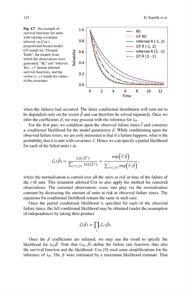
Fig. 4.7 An example of
survival functions for units
with varying covariates
inferred via Cox’s
proportional hazard model.
GT stands for “Ground
Truth”, the models from
which the observations were
generated, “R 0 ” and “inferred
R[x, y]” denote inferred
survival functions, and the
vector [x, y] stands for values
of the covariates
when the failures had occurred. The latter conditional distribution will turn out to
be dependent only on the vector
β and can therefore be solved separately. Once we
infer the coefficients β, we may proceed with the inference for λ 0 .
For the first part, we condition upon the observed failure times
t and construct
a conditional likelihood for the model parameters β. While conditioning upon the
observed failure times, we are only interested in that if a failure happens, what is the
probability that it is unit with covariates
x. Hence we can specify a partial likelihood
for each of the failed units i as
L i (
β) =
λ(t i || x i )
j :t j ≥t i
λ(t i || x j )
=
exp
x i
β
j :t j ≥t i
exp
x j
β
,
where the normalisation is carried over all the units at risk at time of the failure of
the i-th unit. This treatment allowed Cox to also apply his method for censored
observations. The censored observations come into play via the normalisation
constant by decreasing the amount of units at risk at observed failure times. The
equations for conditional likelihood remain the same in such case.
Once the partial conditional likelihood is specified for each of the observed
failure times, the full conditional likelihood may be obtained (under the assumption
of independence) by taking their product
L(
β) =
i
L i (
β).
Once the β coefficients are inferred, we may use the result to specify the
likelihood for λ 0 |
β. Note that (λ 0 ,
β) define the failure rate function, thus also
the survival function and the likelihood. Cox [9] used some simplifications for the
inference of λ 0 . The β were estimated by a maximum likelihood estimate. That
D. Krpelík et al.
Fig. 4.7 An example of
survival functions for units
with varying covariates
inferred via Cox’s
proportional hazard model.
GT stands for “Ground
Truth”, the models from
which the observations were
generated, “R 0 ” and “inferred
R[x, y]” denote inferred
survival functions, and the
vector [x, y] stands for values
of the covariates
when the failures had occurred. The latter conditional distribution will turn out to
be dependent only on the vector
β and can therefore be solved separately. Once we
infer the coefficients β, we may proceed with the inference for λ 0 .
For the first part, we condition upon the observed failure times
t and construct
a conditional likelihood for the model parameters β. While conditioning upon the
observed failure times, we are only interested in that if a failure happens, what is the
probability that it is unit with covariates
x. Hence we can specify a partial likelihood
for each of the failed units i as
L i (
β) =
λ(t i || x i )
j :t j ≥t i
λ(t i || x j )
=
exp
x i
β
j :t j ≥t i
exp
x j
β
,
where the normalisation is carried over all the units at risk at time of the failure of
the i-th unit. This treatment allowed Cox to also apply his method for censored
observations. The censored observations come into play via the normalisation
constant by decreasing the amount of units at risk at observed failure times. The
equations for conditional likelihood remain the same in such case.
Once the partial conditional likelihood is specified for each of the observed
failure times, the full conditional likelihood may be obtained (under the assumption
of independence) by taking their product
L(
β) =
i
L i (
β).
Once the β coefficients are inferred, we may use the result to specify the
likelihood for λ 0 |
β. Note that (λ 0 ,
β) define the failure rate function, thus also
the survival function and the likelihood. Cox [9] used some simplifications for the
inference of λ 0 . The β were estimated by a maximum likelihood estimate. That