

4 Reliability Theory
131
Once we obtain the posterior distribution for the model parameters ((B, C) or
(p, β, α V 0 )) (in the Bayesian framework), we can propagate it directly to obtain the
distribution for the TTF at the working level,
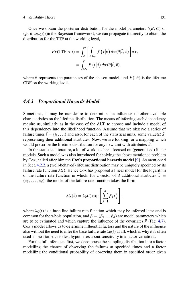
P r(TTF < t) =
t
0
Ω θ
f
x
θ
dπ(θ| t,
v)
dx,
=
Ω θ
F
t
θ
dπ(θ| t,
v).
where θ represents the parameters of the chosen model, and F (.|θ) is the lifetime
CDF on the working level.
4.4.3 Proportional Hazards Model
Sometimes, it may be our desire to determine the influence of other available
characteristics on the lifetime distribution. The means of inferring such dependency
require us, similarly as in the case of the ALT, to choose and include a model of
this dependency into the likelihood function. Assume that we observe a series of
failure times
t = (t 1 , . . .) and also, for each of the statistical units, some value(s)
x i
representing their additional attributes. Now, we are looking for a mapping which
would prescribe the lifetime distribution for any new unit with attributes
x .
In the statistics literature, a lot of work has been focused on (generalised) linear
models. Such a model was also introduced for solving the above mentioned problem
by Cox, called after him the Cox’s proportional hazards model [9]. As mentioned
in Sect. 4.2.2, a (well-behaved) lifetime distribution may be uniquely specified by its
failure rate function λ(t). Hence Cox has proposed a linear model for the logarithm
of the failure rate function in which, for a vector of d additional attributes
x =
(x 1 , . . . , x d ), the model of the failure rate function takes the form
λ(t|| x) = λ 0 (t) exp
⎡
⎣
d
j =1
β j x
i
j
⎤
⎦ ,
where λ 0 (t) is a base-line failure rate function which may be inferred later and is
common for the whole population, and β = (β 1 . . . β d ) are model parameters which
are to be estimated and which capture the influence of the covariates
x (Fig. 4.7).
Cox’s model allows us to determine influential factors and the nature of the influence
also without the need to infer the base failure rate λ 0 (t) at all, which is why it is often
used in bio-statistics to test hypotheses about sensitivity to a factor variations.
For the full inference, first, we decompose the sampling distribution into a factor
modelling the chance of observing the failures at specified times and a factor
modelling the conditional probability of observing them in specified order given
131
Once we obtain the posterior distribution for the model parameters ((B, C) or
(p, β, α V 0 )) (in the Bayesian framework), we can propagate it directly to obtain the
distribution for the TTF at the working level,
P r(TTF < t) =
t
0
Ω θ
f
x
θ
dπ(θ| t,
v)
dx,
=
Ω θ
F
t
θ
dπ(θ| t,
v).
where θ represents the parameters of the chosen model, and F (.|θ) is the lifetime
CDF on the working level.
4.4.3 Proportional Hazards Model
Sometimes, it may be our desire to determine the influence of other available
characteristics on the lifetime distribution. The means of inferring such dependency
require us, similarly as in the case of the ALT, to choose and include a model of
this dependency into the likelihood function. Assume that we observe a series of
failure times
t = (t 1 , . . .) and also, for each of the statistical units, some value(s)
x i
representing their additional attributes. Now, we are looking for a mapping which
would prescribe the lifetime distribution for any new unit with attributes
x .
In the statistics literature, a lot of work has been focused on (generalised) linear
models. Such a model was also introduced for solving the above mentioned problem
by Cox, called after him the Cox’s proportional hazards model [9]. As mentioned
in Sect. 4.2.2, a (well-behaved) lifetime distribution may be uniquely specified by its
failure rate function λ(t). Hence Cox has proposed a linear model for the logarithm
of the failure rate function in which, for a vector of d additional attributes
x =
(x 1 , . . . , x d ), the model of the failure rate function takes the form
λ(t|| x) = λ 0 (t) exp
⎡
⎣
d
j =1
β j x
i
j
⎤
⎦ ,
where λ 0 (t) is a base-line failure rate function which may be inferred later and is
common for the whole population, and β = (β 1 . . . β d ) are model parameters which
are to be estimated and which capture the influence of the covariates
x (Fig. 4.7).
Cox’s model allows us to determine influential factors and the nature of the influence
also without the need to infer the base failure rate λ 0 (t) at all, which is why it is often
used in bio-statistics to test hypotheses about sensitivity to a factor variations.
For the full inference, first, we decompose the sampling distribution into a factor
modelling the chance of observing the failures at specified times and a factor
modelling the conditional probability of observing them in specified order given