

5.8 The First Space Flight Test and Its Results
393
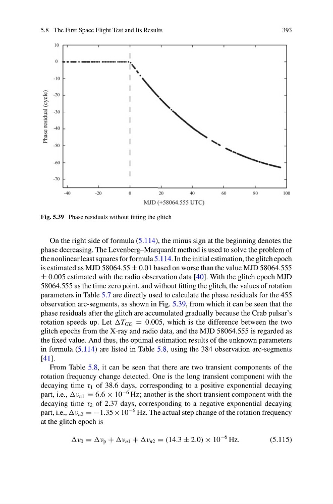
Fig. 5.39 Phase residuals without fitting the glitch
On the right side of formula (5.114), the minus sign at the beginning denotes the
phase decreasing. The Levenberg–Marquardt method is used to solve the problem of
the nonlinear least squares for formula 5.114. In the initial estimation, the glitch epoch
is estimated as MJD 58064.55 ± 0.01 based on worse than the value MJD 58064.555
± 0.005 estimated with the radio observation data [40]. With the glitch epoch MJD
58064.555 as the time zero point, and without fitting the glitch, the values of rotation
parameters in Table 5.7 are directly used to calculate the phase residuals for the 455
observation arc-segments, as shown in Fig. 5.39, from which it can be seen that the
phase residuals after the glitch are accumulated gradually because the Crab pulsar’s
rotation speeds up. Let T GE = 0.005, which is the difference between the two
glitch epochs from the X-ray and radio data, and the MJD 58064.555 is regarded as
the fixed value. And thus, the optimal estimation results of the unknown parameters
in formula (5.114) are listed in Table 5.8, using the 384 observation arc-segments
[41].
From Table 5.8, it can be seen that there are two transient components of the
rotation frequency change detected. One is the long transient component with the
decaying time τ 1 of 38.6 days, corresponding to a positive exponential decaying
part, i.e., ν n1 = 6.6 × 10
−6 Hz; another is the short transient component with the
decaying time τ 2 of 2.37 days, corresponding to a negative exponential decaying
part, i.e., ν n2 = −1.35 × 10
−6 Hz. The actual step change of the rotation frequency
at the glitch epoch is
ν 0 = ν p + ν n1 + ν n2 = (14.3 ± 2.0) × 10
−6 Hz.
(5.115)
393
Fig. 5.39 Phase residuals without fitting the glitch
On the right side of formula (5.114), the minus sign at the beginning denotes the
phase decreasing. The Levenberg–Marquardt method is used to solve the problem of
the nonlinear least squares for formula 5.114. In the initial estimation, the glitch epoch
is estimated as MJD 58064.55 ± 0.01 based on worse than the value MJD 58064.555
± 0.005 estimated with the radio observation data [40]. With the glitch epoch MJD
58064.555 as the time zero point, and without fitting the glitch, the values of rotation
parameters in Table 5.7 are directly used to calculate the phase residuals for the 455
observation arc-segments, as shown in Fig. 5.39, from which it can be seen that the
phase residuals after the glitch are accumulated gradually because the Crab pulsar’s
rotation speeds up. Let T GE = 0.005, which is the difference between the two
glitch epochs from the X-ray and radio data, and the MJD 58064.555 is regarded as
the fixed value. And thus, the optimal estimation results of the unknown parameters
in formula (5.114) are listed in Table 5.8, using the 384 observation arc-segments
[41].
From Table 5.8, it can be seen that there are two transient components of the
rotation frequency change detected. One is the long transient component with the
decaying time τ 1 of 38.6 days, corresponding to a positive exponential decaying
part, i.e., ν n1 = 6.6 × 10
−6 Hz; another is the short transient component with the
decaying time τ 2 of 2.37 days, corresponding to a negative exponential decaying
part, i.e., ν n2 = −1.35 × 10
−6 Hz. The actual step change of the rotation frequency
at the glitch epoch is
ν 0 = ν p + ν n1 + ν n2 = (14.3 ± 2.0) × 10
−6 Hz.
(5.115)