

5.8 The First Space Flight Test and Its Results
391
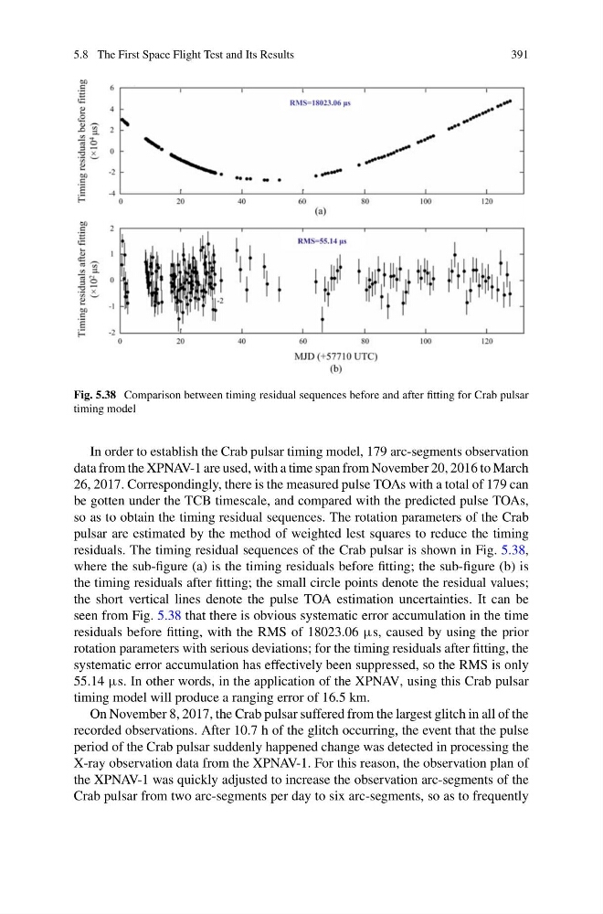
Fig. 5.38 Comparison between timing residual sequences before and after fitting for Crab pulsar
timing model
In order to establish the Crab pulsar timing model, 179 arc-segments observation
data from the XPNAV-1 are used, with a time span from November 20, 2016 to March
26, 2017. Correspondingly, there is the measured pulse TOAs with a total of 179 can
be gotten under the TCB timescale, and compared with the predicted pulse TOAs,
so as to obtain the timing residual sequences. The rotation parameters of the Crab
pulsar are estimated by the method of weighted lest squares to reduce the timing
residuals. The timing residual sequences of the Crab pulsar is shown in Fig. 5.38,
where the sub-figure (a) is the timing residuals before fitting; the sub-figure (b) is
the timing residuals after fitting; the small circle points denote the residual values;
the short vertical lines denote the pulse TOA estimation uncertainties. It can be
seen from Fig. 5.38 that there is obvious systematic error accumulation in the time
residuals before fitting, with the RMS of 18023.06 μs, caused by using the prior
rotation parameters with serious deviations; for the timing residuals after fitting, the
systematic error accumulation has effectively been suppressed, so the RMS is only
55.14 μs. In other words, in the application of the XPNAV, using this Crab pulsar
timing model will produce a ranging error of 16.5 km.
On November 8, 2017, the Crab pulsar suffered from the largest glitch in all of the
recorded observations. After 10.7 h of the glitch occurring, the event that the pulse
period of the Crab pulsar suddenly happened change was detected in processing the
X-ray observation data from the XPNAV-1. For this reason, the observation plan of
the XPNAV-1 was quickly adjusted to increase the observation arc-segments of the
Crab pulsar from two arc-segments per day to six arc-segments, so as to frequently
391
Fig. 5.38 Comparison between timing residual sequences before and after fitting for Crab pulsar
timing model
In order to establish the Crab pulsar timing model, 179 arc-segments observation
data from the XPNAV-1 are used, with a time span from November 20, 2016 to March
26, 2017. Correspondingly, there is the measured pulse TOAs with a total of 179 can
be gotten under the TCB timescale, and compared with the predicted pulse TOAs,
so as to obtain the timing residual sequences. The rotation parameters of the Crab
pulsar are estimated by the method of weighted lest squares to reduce the timing
residuals. The timing residual sequences of the Crab pulsar is shown in Fig. 5.38,
where the sub-figure (a) is the timing residuals before fitting; the sub-figure (b) is
the timing residuals after fitting; the small circle points denote the residual values;
the short vertical lines denote the pulse TOA estimation uncertainties. It can be
seen from Fig. 5.38 that there is obvious systematic error accumulation in the time
residuals before fitting, with the RMS of 18023.06 μs, caused by using the prior
rotation parameters with serious deviations; for the timing residuals after fitting, the
systematic error accumulation has effectively been suppressed, so the RMS is only
55.14 μs. In other words, in the application of the XPNAV, using this Crab pulsar
timing model will produce a ranging error of 16.5 km.
On November 8, 2017, the Crab pulsar suffered from the largest glitch in all of the
recorded observations. After 10.7 h of the glitch occurring, the event that the pulse
period of the Crab pulsar suddenly happened change was detected in processing the
X-ray observation data from the XPNAV-1. For this reason, the observation plan of
the XPNAV-1 was quickly adjusted to increase the observation arc-segments of the
Crab pulsar from two arc-segments per day to six arc-segments, so as to frequently