

84
6 Three-Body Approach to Structural Properties …
p −
9 Li interaction is essentially the same as that of n−
9 Li system. With this proviso,
we can then use the parameters of n−
9 Li potential and predict the low-energy observables as influenced by the presence of Coulomb force in p−
9 Li scattering. Employing
the potential of Eqs. (6.25)–(6.28), we solve the Schrodinger equation for p −
9 Li
system and compute the scattering amplitude in both s- and p-waves. From this, we
can then predict the values of the low-energy observables for p −
9 Li scattering as
scattering length a sc = 23.98 fm and effective range r sc = 1.143 fm in the case of
s-state interaction while the position and width of the p-wave p −
9 Li resonance are
found to be E r = 2.42 MeV and = 6.56 MeV. Thus, it appears that Coulomb force
plays a significant role at such low energies in so far as it affects the values of these
observables considerably.
For Gamow–Teller β-decay of
11 Li involving the halo neutron pair in T = 1 and
S = 0 state, one of the neutrons transforms into a proton resulting in n–p pair in T
= 0 and S = 1 state. For this spin-triplet state of the halo n–p pair, we choose the
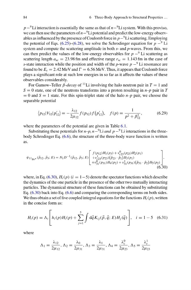
separable potential
p 12 |V 12 | p
12
= −
λ 12
2μ 12
f ( p 12 ) f
p
12
, f ( p) =
1
p 2 + β
2
12
,
(6.29)
where the parameters of the potential are given in Table 6.1.
Substituting these potentials for n–p, n−
9 Li and p −
9 Li interactions in the threebody Schrodinger Eq. (6.6), the structure of the three-body wave function is written
as.
ψ 11 Be ∗ (
p 12 ,
p 3 ; E) = N 1 D −1 (
p 12 ,
p 3 ; E)
⎡
⎢
⎣
f ( p 12 )H 1 ( p 3 ) + v 0
c23 ( p 23 )H 2 ( p 1 )
+v 1
c23 ( p 23 )
ˆ
p 23 · ˆ
p 1
H 3 ( p 1 )
+v 0
31 ( p 31 )H 4 ( p 2 ) + v 1
31 ( p 31 )
ˆ
p 31 · ˆ
p 2
H 5 ( p 2 )
⎤
⎥
⎦,
(6.30)
where, in Eq. (6.30), H i ( p) (i = 1−5) denote the spectator functions which describe
the dynamics of the one particle in the presence of the other two mutually interacting
particles. The dynamical structure of these functions can be obtained by substituting
Eq. (6.30) back into Eq. (6.6) and comparing the corresponding terms on both sides.
We thus obtain a set of five coupled integral equations for the functions H i ( p), written
in the concise form as:
H i ( p) = i
⎡
⎣ h i ( p)H i ( p) +
5
j=1
d q K i j (
p,
q; E)H j ( q)
⎤
⎦ , i = 1 − 5 (6.31)
where
1 =
λ 12
2μ 12
, , 2 =
λ 0
2μ 31
, , 3 =
λ 1
2μ 31
, , 4 =
λ
0
c
2μ 23
, , 5 =
λ
1
c
2μ 23
6 Three-Body Approach to Structural Properties …
p −
9 Li interaction is essentially the same as that of n−
9 Li system. With this proviso,
we can then use the parameters of n−
9 Li potential and predict the low-energy observables as influenced by the presence of Coulomb force in p−
9 Li scattering. Employing
the potential of Eqs. (6.25)–(6.28), we solve the Schrodinger equation for p −
9 Li
system and compute the scattering amplitude in both s- and p-waves. From this, we
can then predict the values of the low-energy observables for p −
9 Li scattering as
scattering length a sc = 23.98 fm and effective range r sc = 1.143 fm in the case of
s-state interaction while the position and width of the p-wave p −
9 Li resonance are
found to be E r = 2.42 MeV and = 6.56 MeV. Thus, it appears that Coulomb force
plays a significant role at such low energies in so far as it affects the values of these
observables considerably.
For Gamow–Teller β-decay of
11 Li involving the halo neutron pair in T = 1 and
S = 0 state, one of the neutrons transforms into a proton resulting in n–p pair in T
= 0 and S = 1 state. For this spin-triplet state of the halo n–p pair, we choose the
separable potential
p 12 |V 12 | p
12
= −
λ 12
2μ 12
f ( p 12 ) f
p
12
, f ( p) =
1
p 2 + β
2
12
,
(6.29)
where the parameters of the potential are given in Table 6.1.
Substituting these potentials for n–p, n−
9 Li and p −
9 Li interactions in the threebody Schrodinger Eq. (6.6), the structure of the three-body wave function is written
as.
ψ 11 Be ∗ (
p 12 ,
p 3 ; E) = N 1 D −1 (
p 12 ,
p 3 ; E)
⎡
⎢
⎣
f ( p 12 )H 1 ( p 3 ) + v 0
c23 ( p 23 )H 2 ( p 1 )
+v 1
c23 ( p 23 )
ˆ
p 23 · ˆ
p 1
H 3 ( p 1 )
+v 0
31 ( p 31 )H 4 ( p 2 ) + v 1
31 ( p 31 )
ˆ
p 31 · ˆ
p 2
H 5 ( p 2 )
⎤
⎥
⎦,
(6.30)
where, in Eq. (6.30), H i ( p) (i = 1−5) denote the spectator functions which describe
the dynamics of the one particle in the presence of the other two mutually interacting
particles. The dynamical structure of these functions can be obtained by substituting
Eq. (6.30) back into Eq. (6.6) and comparing the corresponding terms on both sides.
We thus obtain a set of five coupled integral equations for the functions H i ( p), written
in the concise form as:
H i ( p) = i
⎡
⎣ h i ( p)H i ( p) +
5
j=1
d q K i j (
p,
q; E)H j ( q)
⎤
⎦ , i = 1 − 5 (6.31)
where
1 =
λ 12
2μ 12
, , 2 =
λ 0
2μ 31
, , 3 =
λ 1
2μ 31
, , 4 =
λ
0
c
2μ 23
, , 5 =
λ
1
c
2μ 23