

96
6 Three-Body Approach to Structural Properties …
between the two would increase as p increases. To express λ
−1
c in terms of n–c
scattering length, we have the relation
1
a nc
=
β 1
2
−
β
4
1
2π 2 λ c
or λ
−1
c =
π
2
β
3
1
1 −
2
a nc β 1
Thus,
τ
−1
c = 2a
⎡
⎢
⎢
⎢
⎣
1 −
2
a nc β 1
−
1
1 +
2a
p 2
4c
+ ε 3
2
⎤
⎥
⎥
⎥
⎦
(6.59)
Clearly, so as long as a nc is negative (representing a virtual state) and the third
term is always smaller than the first term, there is hardly any possibility of making
τ
−1
c
→ 0 or τ c → ∞, except when a nc approaches a large value and ε 3 goes to
the zero limit. This is precisely what has been demonstrated through the numerical
analysis. On the other hand, if the binary sub-system is bound corresponding to a
positive scattering length, there is a clear possibility of reducing τ
−1
c or allowing τ c
to be large enough.
6.6 Occurrence of Efimov States in 20 C
A typical example in this case is
20 C considered as a bound system of n–n
18 C, where
n−
18C is known to be bound with binding energy 160 ± 100 keV [91]. In view of
the experimental uncertainties in the determination of the binding energy, we have
carried out the calculations for a range of n −
18 C binding energies varying from 60
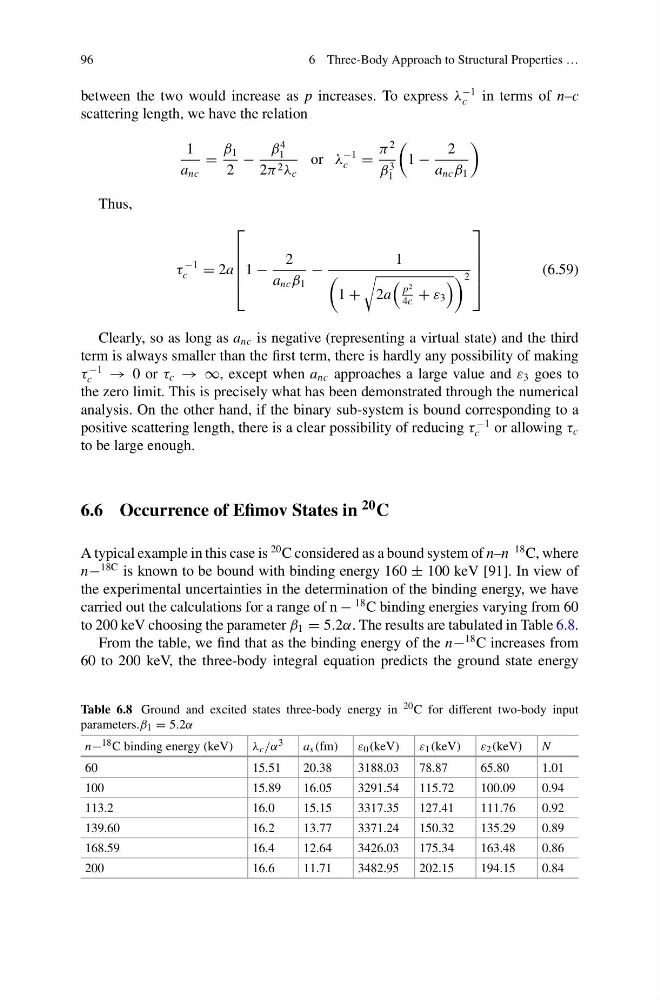
to 200 keV choosing the parameter β 1 = 5.2α. The results are tabulated in Table 6.8.
From the table, we find that as the binding energy of the n−
18 C increases from
60 to 200 keV, the three-body integral equation predicts the ground state energy
Table 6.8 Ground and excited states three-body energy in 20 C for different two-body input
parameters.β 1 = 5.2α
n− 18 C binding energy (keV)
λ c /α 3
a s (fm)
ε 0 (keV)
ε 1 (keV)
ε 2 (keV)
N
60
15.51
20.38
3188.03
78.87
65.80
1.01
100
15.89
16.05
3291.54
115.72
100.09
0.94
113.2
16.0
15.15
3317.35
127.41
111.76
0.92
139.60
16.2
13.77
3371.24
150.32
135.29
0.89
168.59
16.4
12.64
3426.03
175.34
163.48
0.86
200
16.6
11.71
3482.95
202.15
194.15
0.84
6 Three-Body Approach to Structural Properties …
between the two would increase as p increases. To express λ
−1
c in terms of n–c
scattering length, we have the relation
1
a nc
=
β 1
2
−
β
4
1
2π 2 λ c
or λ
−1
c =
π
2
β
3
1
1 −
2
a nc β 1
Thus,
τ
−1
c = 2a
⎡
⎢
⎢
⎢
⎣
1 −
2
a nc β 1
−
1
1 +
2a
p 2
4c
+ ε 3
2
⎤
⎥
⎥
⎥
⎦
(6.59)
Clearly, so as long as a nc is negative (representing a virtual state) and the third
term is always smaller than the first term, there is hardly any possibility of making
τ
−1
c
→ 0 or τ c → ∞, except when a nc approaches a large value and ε 3 goes to
the zero limit. This is precisely what has been demonstrated through the numerical
analysis. On the other hand, if the binary sub-system is bound corresponding to a
positive scattering length, there is a clear possibility of reducing τ
−1
c or allowing τ c
to be large enough.
6.6 Occurrence of Efimov States in 20 C
A typical example in this case is
20 C considered as a bound system of n–n
18 C, where
n−
18C is known to be bound with binding energy 160 ± 100 keV [91]. In view of
the experimental uncertainties in the determination of the binding energy, we have
carried out the calculations for a range of n −
18 C binding energies varying from 60
to 200 keV choosing the parameter β 1 = 5.2α. The results are tabulated in Table 6.8.
From the table, we find that as the binding energy of the n−
18 C increases from
60 to 200 keV, the three-body integral equation predicts the ground state energy
Table 6.8 Ground and excited states three-body energy in 20 C for different two-body input
parameters.β 1 = 5.2α
n− 18 C binding energy (keV)
λ c /α 3
a s (fm)
ε 0 (keV)
ε 1 (keV)
ε 2 (keV)
N
60
15.51
20.38
3188.03
78.87
65.80
1.01
100
15.89
16.05
3291.54
115.72
100.09
0.94
113.2
16.0
15.15
3317.35
127.41
111.76
0.92
139.60
16.2
13.77
3371.24
150.32
135.29
0.89
168.59
16.4
12.64
3426.03
175.34
163.48
0.86
200
16.6
11.71
3482.95
202.15
194.15
0.84