

6.4 Search for Efimov States in Halo Nuclei like 14 Be, 19 B, 22 C and 20 C
9 5
same n–n interaction, the three-body equation predicts the ground state energy of the
22 C nucleus as 1120 keV which is in excellent agreement with the experimentally
determined value [91]. However, here again the input two-body potential does not
allow the three-body equation to admit any solution for the occurrence of the excited
states near the breakup threshold. It is only by changing the parameters of the n−
20 C
potential so as to reduce the excitation energy to a few keV or corresponding to
scattering length to about a hundred Fermi that the Efimov region begins to develop
and the excited states appear for the
22 C system.
6.5 Theoretical Analysis/Interpretation for the Efimov
States from the Model Equation
Having seen quantitatively the general trend for the appearance of Efimov states
in some specific cases, for Borromean-type halo nuclei, it would be instructive to
investigate from analytical considerations to see how far such a behavior is universal.
For this, it is important to realize that the factors which are crucial in governing the
dynamics of binary systems and which play a significant role in describing the kernels
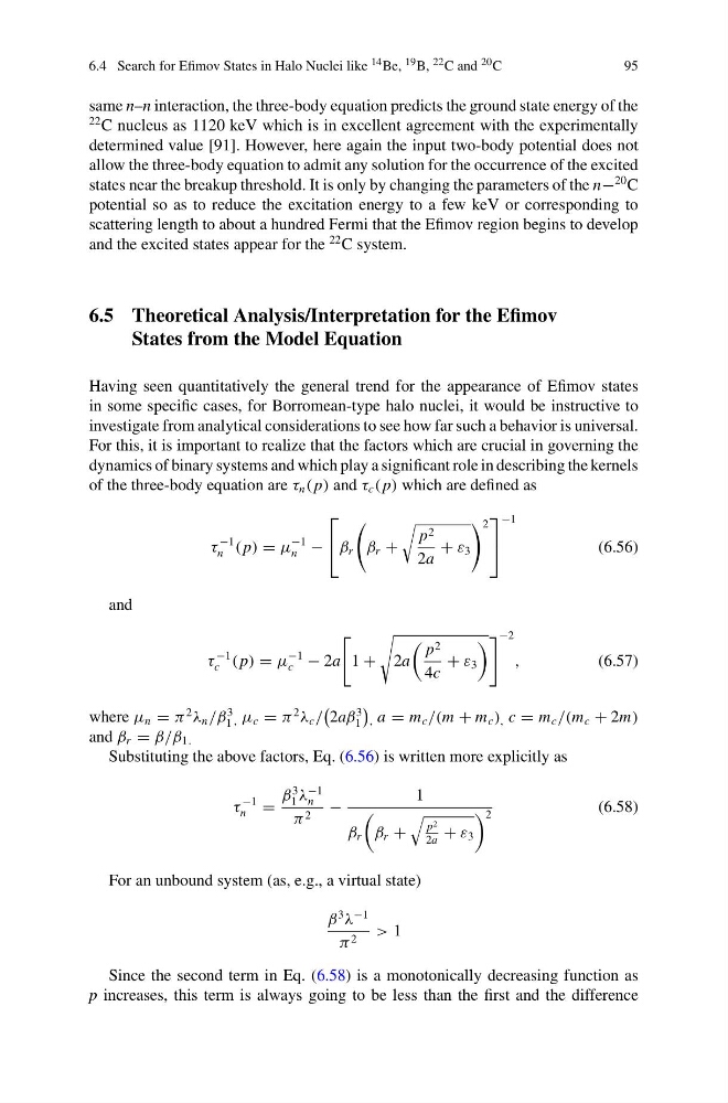
of the three-body equation are τ n ( p) and τ c ( p) which are defined as
τ
−1
n ( p) = μ
−1
n −
⎡
⎣ β r
β r +
p 2
2a
+ ε 3
2
⎤
⎦
−1
(6.56)
and
τ
−1
c ( p) = μ
−1
c − 2a
1 +
2a
p 2
4c
+ ε 3
−2
,
(6.57)
where μ n = π
2
λ n /β
3
1 , μ c = π
2
λ c /
2aβ
3
1
, a = m c /(m + m c ) , c = m c /(m c + 2m)
and β r = β/β 1.
Substituting the above factors, Eq. (6.56) is written more explicitly as
τ
−1
n =
β
3
1 λ
−1
n
π 2 −
1
β r
β r +
p 2
2a
+ ε 3
2
(6.58)
For an unbound system (as, e.g., a virtual state)
β
3
λ
−1
π 2 > 1
Since the second term in Eq. (6.58) is a monotonically decreasing function as
p increases, this term is always going to be less than the first and the difference
9 5
same n–n interaction, the three-body equation predicts the ground state energy of the
22 C nucleus as 1120 keV which is in excellent agreement with the experimentally
determined value [91]. However, here again the input two-body potential does not
allow the three-body equation to admit any solution for the occurrence of the excited
states near the breakup threshold. It is only by changing the parameters of the n−
20 C
potential so as to reduce the excitation energy to a few keV or corresponding to
scattering length to about a hundred Fermi that the Efimov region begins to develop
and the excited states appear for the
22 C system.
6.5 Theoretical Analysis/Interpretation for the Efimov
States from the Model Equation
Having seen quantitatively the general trend for the appearance of Efimov states
in some specific cases, for Borromean-type halo nuclei, it would be instructive to
investigate from analytical considerations to see how far such a behavior is universal.
For this, it is important to realize that the factors which are crucial in governing the
dynamics of binary systems and which play a significant role in describing the kernels
of the three-body equation are τ n ( p) and τ c ( p) which are defined as
τ
−1
n ( p) = μ
−1
n −
⎡
⎣ β r
β r +
p 2
2a
+ ε 3
2
⎤
⎦
−1
(6.56)
and
τ
−1
c ( p) = μ
−1
c − 2a
1 +
2a
p 2
4c
+ ε 3
−2
,
(6.57)
where μ n = π
2
λ n /β
3
1 , μ c = π
2
λ c /
2aβ
3
1
, a = m c /(m + m c ) , c = m c /(m c + 2m)
and β r = β/β 1.
Substituting the above factors, Eq. (6.56) is written more explicitly as
τ
−1
n =
β
3
1 λ
−1
n
π 2 −
1
β r
β r +
p 2
2a
+ ε 3
2
(6.58)
For an unbound system (as, e.g., a virtual state)
β
3
λ
−1
π 2 > 1
Since the second term in Eq. (6.58) is a monotonically decreasing function as
p increases, this term is always going to be less than the first and the difference