

b
P B 1
ð Þu 1 ¼
1
4
ð1Þð1Þu 1 þ ðÀ1ÞðÀ1Þu 3 þ ð1Þð1Þu 3 þ ðÀ1ÞðÀ1Þu 1
½
¼ N u 1 þ u 3
½
b
P B 1
ð Þu 2 ¼
1
4
ð1Þð1Þu 2 þ ðÀ1ÞðÀ1Þu 2 þ ð1Þð1Þu 2 þ ðÀ1ÞðÀ1Þu 2
½
¼ u 2
These two eigenfunctions with identical symmetry can mix as
w 1 ¼ au 1 þ bu 2 þ au 3
w 2 ¼ a
0
u 1 À b
0
u 2 þ a
0
u 3
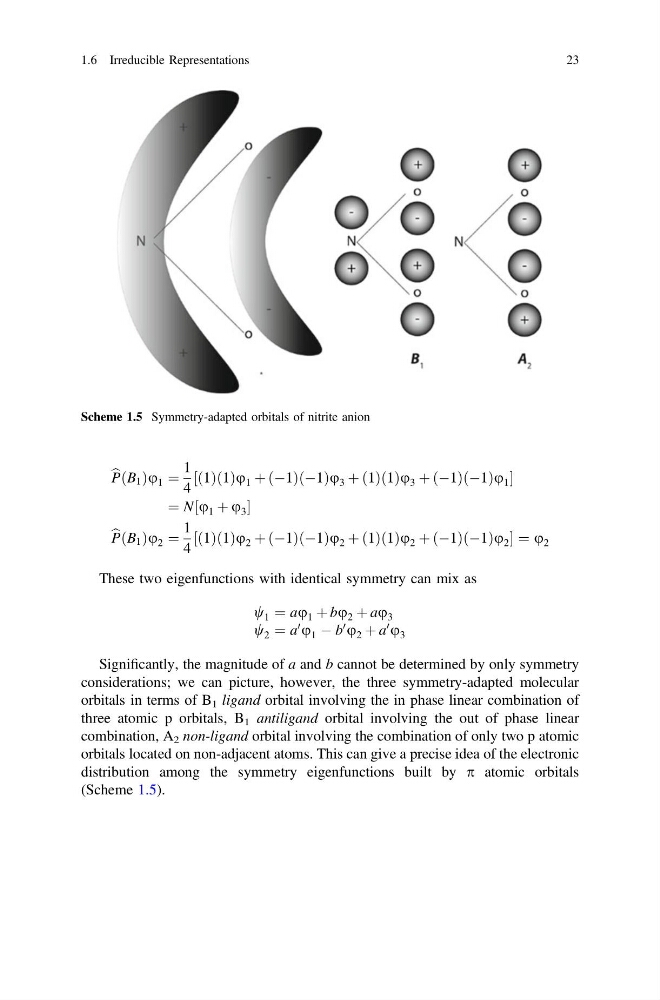
Significantly, the magnitude of a and b cannot be determined by only symmetry
considerations; we can picture, however, the three symmetry-adapted molecular
orbitals in terms of B 1 ligand orbital involving the in phase linear combination of
three atomic p orbitals, B 1 antiligand orbital involving the out of phase linear
combination, A 2 non-ligand orbital involving the combination of only two p atomic
orbitals located on non-adjacent atoms. This can give a precise idea of the electronic
distribution among the symmetry eigenfunctions built by p atomic orbitals
(Scheme 1.5).
Scheme 1.5 Symmetry-adapted orbitals of nitrite anion
1.6 Irreducible Representations
23
P B 1
ð Þu 1 ¼
1
4
ð1Þð1Þu 1 þ ðÀ1ÞðÀ1Þu 3 þ ð1Þð1Þu 3 þ ðÀ1ÞðÀ1Þu 1
½
¼ N u 1 þ u 3
½
b
P B 1
ð Þu 2 ¼
1
4
ð1Þð1Þu 2 þ ðÀ1ÞðÀ1Þu 2 þ ð1Þð1Þu 2 þ ðÀ1ÞðÀ1Þu 2
½
¼ u 2
These two eigenfunctions with identical symmetry can mix as
w 1 ¼ au 1 þ bu 2 þ au 3
w 2 ¼ a
0
u 1 À b
0
u 2 þ a
0
u 3
Significantly, the magnitude of a and b cannot be determined by only symmetry
considerations; we can picture, however, the three symmetry-adapted molecular
orbitals in terms of B 1 ligand orbital involving the in phase linear combination of
three atomic p orbitals, B 1 antiligand orbital involving the out of phase linear
combination, A 2 non-ligand orbital involving the combination of only two p atomic
orbitals located on non-adjacent atoms. This can give a precise idea of the electronic
distribution among the symmetry eigenfunctions built by p atomic orbitals
(Scheme 1.5).
Scheme 1.5 Symmetry-adapted orbitals of nitrite anion
1.6 Irreducible Representations
23