

E1C12 09/14/2010
13:54:15 Page 554
Example 12.7
Consider the second-order system described in Example 12.6. Plot the open loop response of the
system to a step-change in input for damping ratios of 0.3 and 1.3.
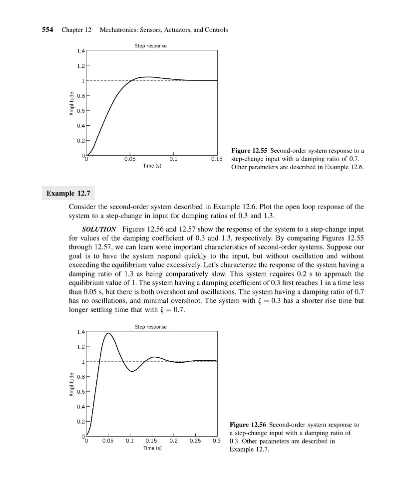
SOLUTION Figures 12.56 and 12.57 show the response of the system to a step-change input
for values of the damping coefficient of 0.3 and 1.3, respectively. By comparing Figures 12.55
through 12.57, we can learn some important characteristics of second-order systems. Suppose our
goal is to have the system respond quickly to the input, but without oscillation and without
exceeding the equilibrium value excessively. Let’s characterize the response of the system having a
damping ratio of 1.3 as being comparatively slow. This system requires 0.2 s to approach the
equilibrium value of 1. The system having a damping coefficient of 0.3 first reaches 1 in a time less
than 0.05 s, but there is both overshoot and oscillations. The system having a damping ratio of 0.7
has no oscillations, and minimal overshoot. The system with z ¼ 0:3 has a shorter rise time but
longer settling time that with z ¼ 0:7.
0
0.2
0.4
0.6
0.8
1
1.2
1.4
0.15
0.1
0.05
0
Time (s)
Step response
Amplitude
Figure 12.55 Second-order system response to a
step-change input with a damping ratio of 0.7.
Other parameters are described in Example 12.6.
0
0.2
0.4
0.6
0.8
1
1.2
1.4
0.25
0.2
0.05
0.3
0.1
0.15
0
Time (s)
Step response
Amplitude
Figure 12.56 Second-order system response to
a step-change input with a damping ratio of
0.3. Other parameters are described in
Example 12.7.
554 Chapter 12 Mechatronics: Sensors, Actuators, and Controls
13:54:15 Page 554
Example 12.7
Consider the second-order system described in Example 12.6. Plot the open loop response of the
system to a step-change in input for damping ratios of 0.3 and 1.3.
SOLUTION Figures 12.56 and 12.57 show the response of the system to a step-change input
for values of the damping coefficient of 0.3 and 1.3, respectively. By comparing Figures 12.55
through 12.57, we can learn some important characteristics of second-order systems. Suppose our
goal is to have the system respond quickly to the input, but without oscillation and without
exceeding the equilibrium value excessively. Let’s characterize the response of the system having a
damping ratio of 1.3 as being comparatively slow. This system requires 0.2 s to approach the
equilibrium value of 1. The system having a damping coefficient of 0.3 first reaches 1 in a time less
than 0.05 s, but there is both overshoot and oscillations. The system having a damping ratio of 0.7
has no oscillations, and minimal overshoot. The system with z ¼ 0:3 has a shorter rise time but
longer settling time that with z ¼ 0:7.
0
0.2
0.4
0.6
0.8
1
1.2
1.4
0.15
0.1
0.05
0
Time (s)
Step response
Amplitude
Figure 12.55 Second-order system response to a
step-change input with a damping ratio of 0.7.
Other parameters are described in Example 12.6.
0
0.2
0.4
0.6
0.8
1
1.2
1.4
0.25
0.2
0.05
0.3
0.1
0.15
0
Time (s)
Step response
Amplitude
Figure 12.56 Second-order system response to
a step-change input with a damping ratio of
0.3. Other parameters are described in
Example 12.7.
554 Chapter 12 Mechatronics: Sensors, Actuators, and Controls