

E1C12 09/14/2010
13:54:15 Page 553
Proportional Integral-Derivative Control of a Second-Order System
Consider a spring-mass-damper system such as the one described in Figure 3.3. The governing
equation describing the position of the mass as a function of time for a given forcing function
f(t) is
1
v 2
n
d
2
y
dt 2 þ
2z
v n
dy
dt
þ y ¼ f ðtÞ
ð 12:60Þ
This system and the governing equation serve as a model to demonstrate the properties of
proportional integral-derivative (PID) control when applied to a second-order system.
The goal is to apply a step change in input to the system, and have the mass move to the new
equilibrium position; in other words, the ideal response of the system would be a step-change. Our
first objective is to review the response of the second-order system without a controller in place. The
behavior of the system is examined in two examples.
Example 12.6
A spring-mass-damper system has mass of 2 kg, a spring constant of 7900 N/m, and a damping
coefficient of 176 kg/s. Plot the open loop time response of this system to a step-change input in
force.
ASSUMPTIONS The initial conditions for velocity,
dy
dt
, and position, y, are zero.
SOLUTION Although, the solution to this example could be determined from the results in
Chapter 3, we will determine the response using Laplace transforms. Taking the Laplace transform
of Equation 12.60 yields
1
v 2
n
s
2
Y s
ð Þ þ
2z
v n
sY s
ð Þ þ Y s
ð Þ ¼ KF s
ð Þ
ð12:61Þ
For the mass, spring constant, and damping ratio given in the problem statement, we compute
the natural frequency and damping ratio as
v n ¼
ffiffiffiffi
k
m
r
¼
ffiffiffiffiffiffiffiffiffiffi
7900
2
r
¼ 62:85 rad=s and z ¼
c
2
ffiffiffiffiffiffi ffi
km
p
¼
176
2
ffiffiffiffiffiffiffiffiffiffiffiffiffiffiffiffiffiffi
7900 Â 2
p
¼ 0:7
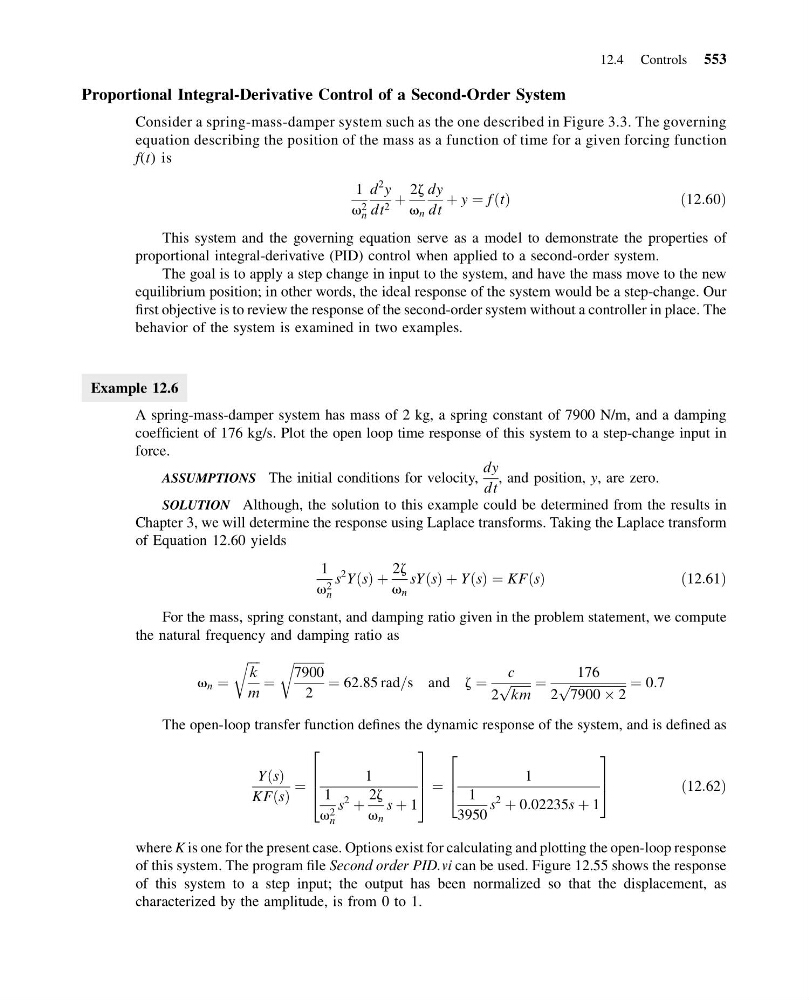
The open-loop transfer function defines the dynamic response of the system, and is defined as
Y s
ð Þ
KF s
ð Þ
¼
1
1
v 2
n
s
2
þ
2z
v n
s þ 1
2
6
6
4
3
7
7
5 ¼
1
1
3950
s
2
þ 0:02235s þ 1
2
6
4
3
7
5
ð12:62Þ
where K is one for the present case. Options exist for calculating and plotting the open-loop response
of this system. The program file Second order PID.vi can be used. Figure 12.55 shows the response
of this system to a step input; the output has been normalized so that the displacement, as
characterized by the amplitude, is from 0 to 1.
12.4 Controls 553
13:54:15 Page 553
Proportional Integral-Derivative Control of a Second-Order System
Consider a spring-mass-damper system such as the one described in Figure 3.3. The governing
equation describing the position of the mass as a function of time for a given forcing function
f(t) is
1
v 2
n
d
2
y
dt 2 þ
2z
v n
dy
dt
þ y ¼ f ðtÞ
ð 12:60Þ
This system and the governing equation serve as a model to demonstrate the properties of
proportional integral-derivative (PID) control when applied to a second-order system.
The goal is to apply a step change in input to the system, and have the mass move to the new
equilibrium position; in other words, the ideal response of the system would be a step-change. Our
first objective is to review the response of the second-order system without a controller in place. The
behavior of the system is examined in two examples.
Example 12.6
A spring-mass-damper system has mass of 2 kg, a spring constant of 7900 N/m, and a damping
coefficient of 176 kg/s. Plot the open loop time response of this system to a step-change input in
force.
ASSUMPTIONS The initial conditions for velocity,
dy
dt
, and position, y, are zero.
SOLUTION Although, the solution to this example could be determined from the results in
Chapter 3, we will determine the response using Laplace transforms. Taking the Laplace transform
of Equation 12.60 yields
1
v 2
n
s
2
Y s
ð Þ þ
2z
v n
sY s
ð Þ þ Y s
ð Þ ¼ KF s
ð Þ
ð12:61Þ
For the mass, spring constant, and damping ratio given in the problem statement, we compute
the natural frequency and damping ratio as
v n ¼
ffiffiffiffi
k
m
r
¼
ffiffiffiffiffiffiffiffiffiffi
7900
2
r
¼ 62:85 rad=s and z ¼
c
2
ffiffiffiffiffiffi ffi
km
p
¼
176
2
ffiffiffiffiffiffiffiffiffiffiffiffiffiffiffiffiffiffi
7900 Â 2
p
¼ 0:7
The open-loop transfer function defines the dynamic response of the system, and is defined as
Y s
ð Þ
KF s
ð Þ
¼
1
1
v 2
n
s
2
þ
2z
v n
s þ 1
2
6
6
4
3
7
7
5 ¼
1
1
3950
s
2
þ 0:02235s þ 1
2
6
4
3
7
5
ð12:62Þ
where K is one for the present case. Options exist for calculating and plotting the open-loop response
of this system. The program file Second order PID.vi can be used. Figure 12.55 shows the response
of this system to a step input; the output has been normalized so that the displacement, as
characterized by the amplitude, is from 0 to 1.
12.4 Controls 553