E1C12 09/14/2010
13:54:14 Page 545
With the appropriate initial condition and steady-state output value, this can be written as
Equation 3.6:
G t
ð Þ ¼
y t
ð Þ À y 1
y 0 À y 1
¼ e
Àt=t
where t is the time constant for a first-order system and G(t) is the error fraction
Example 12.4
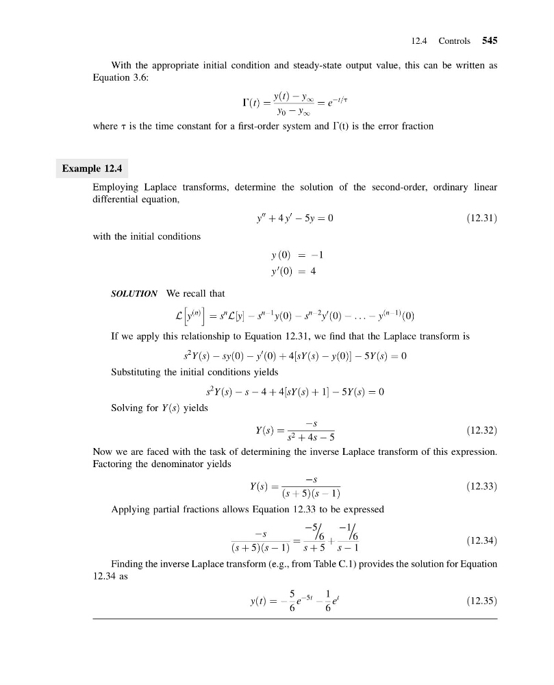
Employing Laplace transforms, determine the solution of the second-order, ordinary linear
differential equation,
y
00
þ 4 y
0
À 5y ¼ 0
ð12:31Þ
with the initial conditions
y 0
ð Þ ¼ À1
y
0 0
ð Þ ¼ 4
SOLUTION We recall that
L y
n
ð Þ
h i
¼ s
n
L y
½ Š À s
nÀ1
y 0
ð Þ À s
nÀ2
y
0 0
ð Þ À . . . À y
nÀ1
ð
Þ 0
ð Þ
If we apply this relationship to Equation 12.31, we find that the Laplace transform is
s
2
Y s
ð Þ À sy 0
ð Þ À y
0 0
ð Þ þ 4 sY s
ð Þ À y 0
ð Þ
½
ŠÀ5Y s
ð Þ ¼ 0
Substituting the initial conditions yields
s
2
Y s
ð Þ À s À 4 þ 4 sY s
ð Þ þ 1
½
ŠÀ5Y s
ð Þ ¼ 0
Solving for Y s
ð Þ yields
Y s
ð Þ ¼
Às
s 2 þ 4s À 5
ð12:32Þ
Now we are faced with the task of determining the inverse Laplace transform of this expression.
Factoring the denominator yields
Y s
ð Þ ¼
Às
s þ 5
ð
Þ s À 1
ð
Þ
ð12:33Þ
Applying partial fractions allows Equation 12.33 to be expressed
Às
s þ 5
ð
Þ s À 1
ð
Þ
¼
À5
= 6
s þ 5
þ
À1
= 6
s À 1
ð12:34Þ
Finding the inverse Laplace transform (e.g., from Table C.1) provides the solution for Equation
12.34 as
y t
ð Þ ¼ À
5
6
e
À5t
À
1
6
e
t
ð12:35Þ
12.4 Controls 545