

E1C12 09/14/2010
13:54:13 Page 543
Many control systems are designed to maintain a specified set point without a dead band;
clearly this is not possible using on–off control. Consider again watering a lawn. Suppose that due to
varying water pressure the lawn was being watered nonuniformly. We might choose to control both
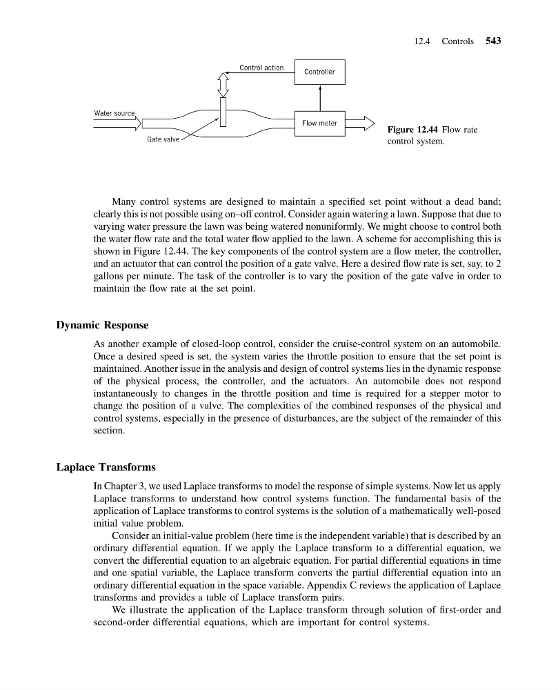
the water flow rate and the total water flow applied to the lawn. A scheme for accomplishing this is
shown in Figure 12.44. The key components of the control system are a flow meter, the controller,
and an actuator that can control the position of a gate valve. Here a desired flow rate is set, say, to 2
gallons per minute. The task of the controller is to vary the position of the gate valve in order to
maintain the flow rate at the set point.
Dynamic Response
As another example of closed-loop control, consider the cruise-control system on an automobile.
Once a desired speed is set, the system varies the throttle position to ensure that the set point is
maintained. Another issue in the analysis and design of control systems lies in the dynamic response
of the physical process, the controller, and the actuators. An automobile does not respond
instantaneously to changes in the throttle position and time is required for a stepper motor to
change the position of a valve. The complexities of the combined responses of the physical and
control systems, especially in the presence of disturbances, are the subject of the remainder of this
section.
Laplace Transforms
In Chapter 3, we used Laplace transforms to model the response of simple systems. Now let us apply
Laplace transforms to understand how control systems function. The fundamental basis of the
application of Laplace transforms to control systems is the solution of a mathematically well-posed
initial value problem.
Consider an initial-value problem (here time is the independent variable) that is described by an
ordinary differential equation. If we apply the Laplace transform to a differential equation, we
convert the differential equation to an algebraic equation. For partial differential equations in time
and one spatial variable, the Laplace transform converts the partial differential equation into an
ordinary differential equation in the space variable. Appendix C reviews the application of Laplace
transforms and provides a table of Laplace transform pairs.
We illustrate the application of the Laplace transform through solution of first-order and
second-order differential equations, which are important for control systems.
Flow meter
Controller
Gate valve
Control action
Water source
Figure 12.44 Flow rate
control system.
12.4 Controls 543
13:54:13 Page 543
Many control systems are designed to maintain a specified set point without a dead band;
clearly this is not possible using on–off control. Consider again watering a lawn. Suppose that due to
varying water pressure the lawn was being watered nonuniformly. We might choose to control both
the water flow rate and the total water flow applied to the lawn. A scheme for accomplishing this is
shown in Figure 12.44. The key components of the control system are a flow meter, the controller,
and an actuator that can control the position of a gate valve. Here a desired flow rate is set, say, to 2
gallons per minute. The task of the controller is to vary the position of the gate valve in order to
maintain the flow rate at the set point.
Dynamic Response
As another example of closed-loop control, consider the cruise-control system on an automobile.
Once a desired speed is set, the system varies the throttle position to ensure that the set point is
maintained. Another issue in the analysis and design of control systems lies in the dynamic response
of the physical process, the controller, and the actuators. An automobile does not respond
instantaneously to changes in the throttle position and time is required for a stepper motor to
change the position of a valve. The complexities of the combined responses of the physical and
control systems, especially in the presence of disturbances, are the subject of the remainder of this
section.
Laplace Transforms
In Chapter 3, we used Laplace transforms to model the response of simple systems. Now let us apply
Laplace transforms to understand how control systems function. The fundamental basis of the
application of Laplace transforms to control systems is the solution of a mathematically well-posed
initial value problem.
Consider an initial-value problem (here time is the independent variable) that is described by an
ordinary differential equation. If we apply the Laplace transform to a differential equation, we
convert the differential equation to an algebraic equation. For partial differential equations in time
and one spatial variable, the Laplace transform converts the partial differential equation into an
ordinary differential equation in the space variable. Appendix C reviews the application of Laplace
transforms and provides a table of Laplace transform pairs.
We illustrate the application of the Laplace transform through solution of first-order and
second-order differential equations, which are important for control systems.
Flow meter
Controller
Gate valve
Control action
Water source
Figure 12.44 Flow rate
control system.
12.4 Controls 543