

E1C09 09/14/2010
15:4:56 Page 412
The analysis can work in one of two ways. In the first approach, the analyzer performs the fast
Fourier transform (FFT) continuously on small blocks of data from which the Doppler frequency is
directly determined. In the second mode, the correlation mode, the sampled signal is correlated with
itself through a mathematical transformation of the form
R j ¼
X n
i¼1
xðiÞxði þ jÞ
ð 9:52Þ
where i refers to the sample value at time t and j to the sample value at time delay Dt. This operation
improves the signal-to-noise ratio (SNR) of the signal; the frequency is determined from the
correlation function and the sample rate. From Equation 9.51, the Doppler frequency can be
converted to a velocity and provided as an output signal. The acquisition and analysis occur rapidly
so that the signal appears nearly continuous in time and with only a short time lag.
All methods output a voltage that is proportional to the instantaneous velocity, which makes
their signal easy to process, or a digital output path to a digital file for signal analysis. At very low
light levels and very few scattering particles, the signal level to noise level can be very low. In such
cases, photon correlation techniques are successful (20,21).
The LDA technique measures velocity at a point. Thus, its probe volume needs to be moved
around to map out the flow field. If the SNR and seeding is good, the LDA can measure timedependent velocities well. The LDA technique is particularly useful where probe blockage effects
render other methods unsuitable, where fluid density and temperature fluctuations occur, or where
environments hostile to physical sensors exist. An extended discussion of LDA techniques can be
found elsewhere (21,22).
Example 9.11
A laser Doppler anemometer made up of a He-Ne laser (l ¼ 632.8 nm) is used to measure the
velocity of water at a point in a flow. A 150-mm lens, with u ¼ 11 degrees, is used to operate
the LDA in a dual-beam mode. If an average Doppler frequency of 1.41 MHz is measured,
estimate the velocity of water.
KNOWN f D ¼ 1:41 MHz
l ¼ 632:8 nm u ¼ 11 degrees
ASSUMPTIONS Scattering particles follow the water exactly.
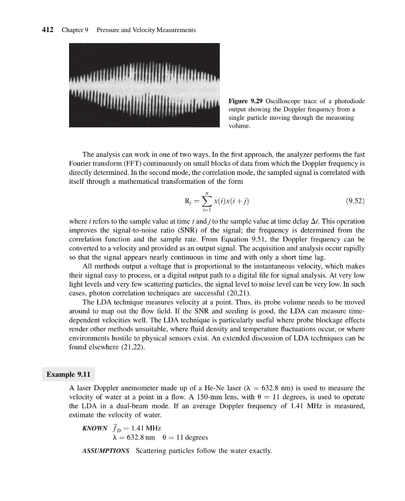
Figure 9.29 Oscilloscope trace of a photodiode
output showing the Doppler frequency from a
single particle moving through the measuring
volume.
412 Chapter 9 Pressure and Velocity Measurements
15:4:56 Page 412
The analysis can work in one of two ways. In the first approach, the analyzer performs the fast
Fourier transform (FFT) continuously on small blocks of data from which the Doppler frequency is
directly determined. In the second mode, the correlation mode, the sampled signal is correlated with
itself through a mathematical transformation of the form
R j ¼
X n
i¼1
xðiÞxði þ jÞ
ð 9:52Þ
where i refers to the sample value at time t and j to the sample value at time delay Dt. This operation
improves the signal-to-noise ratio (SNR) of the signal; the frequency is determined from the
correlation function and the sample rate. From Equation 9.51, the Doppler frequency can be
converted to a velocity and provided as an output signal. The acquisition and analysis occur rapidly
so that the signal appears nearly continuous in time and with only a short time lag.
All methods output a voltage that is proportional to the instantaneous velocity, which makes
their signal easy to process, or a digital output path to a digital file for signal analysis. At very low
light levels and very few scattering particles, the signal level to noise level can be very low. In such
cases, photon correlation techniques are successful (20,21).
The LDA technique measures velocity at a point. Thus, its probe volume needs to be moved
around to map out the flow field. If the SNR and seeding is good, the LDA can measure timedependent velocities well. The LDA technique is particularly useful where probe blockage effects
render other methods unsuitable, where fluid density and temperature fluctuations occur, or where
environments hostile to physical sensors exist. An extended discussion of LDA techniques can be
found elsewhere (21,22).
Example 9.11
A laser Doppler anemometer made up of a He-Ne laser (l ¼ 632.8 nm) is used to measure the
velocity of water at a point in a flow. A 150-mm lens, with u ¼ 11 degrees, is used to operate
the LDA in a dual-beam mode. If an average Doppler frequency of 1.41 MHz is measured,
estimate the velocity of water.
KNOWN f D ¼ 1:41 MHz
l ¼ 632:8 nm u ¼ 11 degrees
ASSUMPTIONS Scattering particles follow the water exactly.
Figure 9.29 Oscilloscope trace of a photodiode
output showing the Doppler frequency from a
single particle moving through the measuring
volume.
412 Chapter 9 Pressure and Velocity Measurements