

E1C09 09/14/2010
15:4:55 Page 402
R
R
L
L f
P m
C vp
P a
E m
E a
C
(a)
(b)
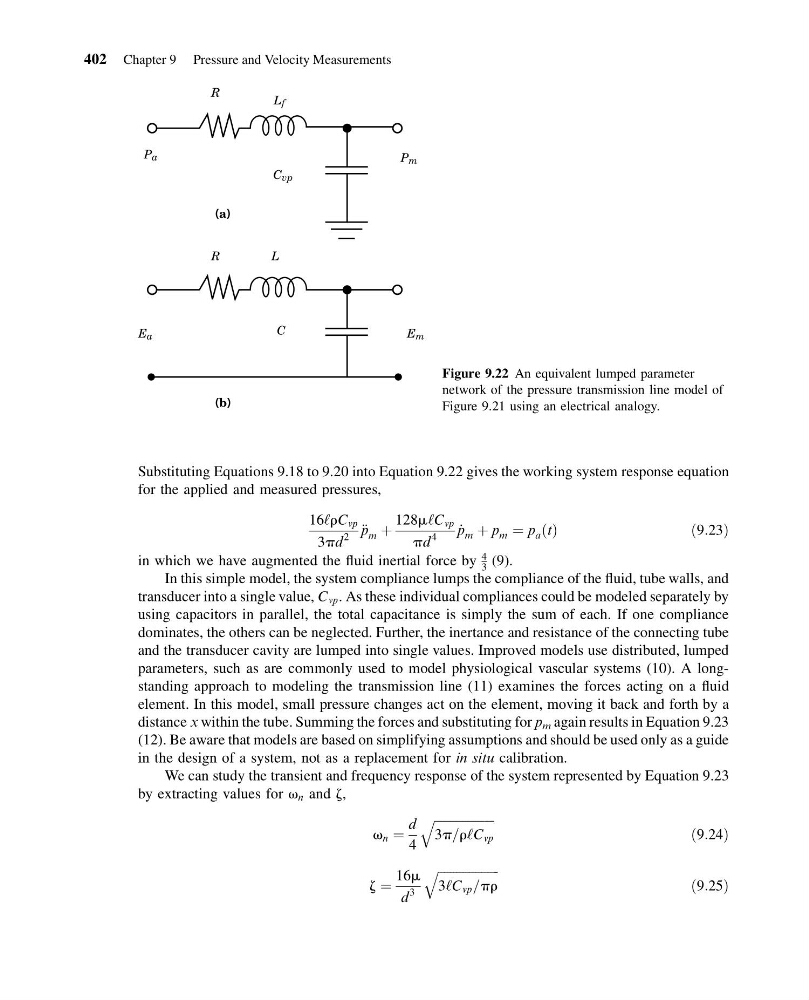
Figure 9.22 An equivalent lumped parameter
network of the pressure transmission line model of
Figure 9.21 using an electrical analogy.
Substituting Equations 9.18 to 9.20 into Equation 9.22 gives the working system response equation
for the applied and measured pressures,
16‘rC vp
3pd
2
€ p m þ
128m‘C vp
pd
4
_
p m þ p m ¼ p a t
ð Þ
ð9:23Þ
in which we have augmented the fluid inertial force by
4
3 (9).
In this simple model, the system compliance lumps the compliance of the fluid, tube walls, and
transducer into a single value, C vp . As these individual compliances could be modeled separately by
using capacitors in parallel, the total capacitance is simply the sum of each. If one compliance
dominates, the others can be neglected. Further, the inertance and resistance of the connecting tube
and the transducer cavity are lumped into single values. Improved models use distributed, lumped
parameters, such as are commonly used to model physiological vascular systems (10). A longstanding approach to modeling the transmission line (11) examines the forces acting on a fluid
element. In this model, small pressure changes act on the element, moving it back and forth by a
distance x within the tube. Summing the forces and substituting for p m again results in Equation 9.23
(12). Be aware that models are based on simplifying assumptions and should be used only as a guide
in the design of a system, not as a replacement for in situ calibration.
We can study the transient and frequency response of the system represented by Equation 9.23
by extracting values for v n and z,
v n ¼
d
4
ffiffiffiffiffiffiffiffiffiffiffiffiffiffiffiffiffiffiffi ffi
3p=r‘C vp
q
ð9:24Þ
z ¼
16m
d
3
ffiffiffiffiffiffiffiffiffiffiffiffiffiffiffiffiffiffiffi ffi
3‘C vp =pr
q
ð9:25Þ
402 Chapter 9 Pressure and Velocity Measurements
15:4:55 Page 402
R
R
L
L f
P m
C vp
P a
E m
E a
C
(a)
(b)
Figure 9.22 An equivalent lumped parameter
network of the pressure transmission line model of
Figure 9.21 using an electrical analogy.
Substituting Equations 9.18 to 9.20 into Equation 9.22 gives the working system response equation
for the applied and measured pressures,
16‘rC vp
3pd
2
€ p m þ
128m‘C vp
pd
4
_
p m þ p m ¼ p a t
ð Þ
ð9:23Þ
in which we have augmented the fluid inertial force by
4
3 (9).
In this simple model, the system compliance lumps the compliance of the fluid, tube walls, and
transducer into a single value, C vp . As these individual compliances could be modeled separately by
using capacitors in parallel, the total capacitance is simply the sum of each. If one compliance
dominates, the others can be neglected. Further, the inertance and resistance of the connecting tube
and the transducer cavity are lumped into single values. Improved models use distributed, lumped
parameters, such as are commonly used to model physiological vascular systems (10). A longstanding approach to modeling the transmission line (11) examines the forces acting on a fluid
element. In this model, small pressure changes act on the element, moving it back and forth by a
distance x within the tube. Summing the forces and substituting for p m again results in Equation 9.23
(12). Be aware that models are based on simplifying assumptions and should be used only as a guide
in the design of a system, not as a replacement for in situ calibration.
We can study the transient and frequency response of the system represented by Equation 9.23
by extracting values for v n and z,
v n ¼
d
4
ffiffiffiffiffiffiffiffiffiffiffiffiffiffiffiffiffiffiffi ffi
3p=r‘C vp
q
ð9:24Þ
z ¼
16m
d
3
ffiffiffiffiffiffiffiffiffiffiffiffiffiffiffiffiffiffiffi ffi
3‘C vp =pr
q
ð9:25Þ
402 Chapter 9 Pressure and Velocity Measurements