

E1C09 09/14/2010
15:4:55 Page 401
where n ¼ 1 for laminar and n ¼ 0.5 for turbulent flows. Hence, Q ¼
1
R
Dp
n .
The resistance of the laminar flow of a newtonian fluid through a circular pipe is R ¼
128m‘
pd
4
,
where m is the fluid viscosity. In electrical systems, it has the analogous meaning as the opposition to
current flow for an imposed voltage potential, such as an electrical resistor.
Compliance describes a measure of the volume change associated with a corresponding
pressure change, such as
C vp ¼ D8=Dp
ð9:20Þ
It is a measure of the flexibility in a structure, component, or substance, and so it is the inverse of the
system stiffness. Compliance is the direct analog to electrical capacitance.
9.8 DESIGN AND INSTALLATION: TRANSMISSION EFFECTS
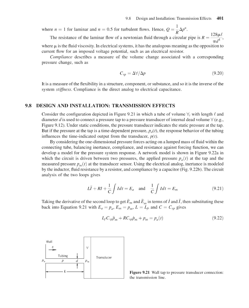
Consider the configuration depicted in Figure 9.21 in which a tube of volume 8 t with length ‘ and
diameter d is used to connect a pressure tap to a pressure transducer of internal dead volume 8 (e.g.,
Figure 9.12). Under static conditions, the pressure transducer indicates the static pressure at the tap.
But if the pressure at the tap is a time-dependent pressure, p a (t), the response behavior of the tubing
influences the time-indicated output from the transducer, p(t).
By considering the one-dimensional pressure forces acting on a lumped mass of fluid within the
connecting tube, balancing inertance, compliance, and resistance against forcing function, we can
develop a model for the pressure system response. A network model is shown in Figure 9.22a in
which the circuit is driven between two pressures, the applied pressure p a ðtÞ at the tap and the
measured pressure p m ðtÞ at the transducer sensor. Using the electrical analog, inertance is modeled
by the inductor, fluid resistance by a resistor, and compliance by a capacitor (Fig. 9.22b). The circuit
analysis of the two loops gives
L €
I þ RI þ
1
C
Z
Idt ¼ E a and
1
C
Z
Idt ¼ E m
ð9:21Þ
Taking the derivative of the second loop to get _
E m and €
E m in terms of _
I and €
I , then substituting these
back into Equation 9.21 with E a ¼ p a , E m ¼ p m , L ¼ L f , and C ¼ C vp gives
L f C vp € p m þ RC vp _
p m þ p m ¼ p a t
ð Þ
ð9:22Þ
Transducer
Tubing
Wall
p m
p a
d
p
x
∀
Figure 9.21 Wall tap to pressure transducer connection:
the transmission line.
9.8 Design and Installation: Transmission Effects 401
15:4:55 Page 401
where n ¼ 1 for laminar and n ¼ 0.5 for turbulent flows. Hence, Q ¼
1
R
Dp
n .
The resistance of the laminar flow of a newtonian fluid through a circular pipe is R ¼
128m‘
pd
4
,
where m is the fluid viscosity. In electrical systems, it has the analogous meaning as the opposition to
current flow for an imposed voltage potential, such as an electrical resistor.
Compliance describes a measure of the volume change associated with a corresponding
pressure change, such as
C vp ¼ D8=Dp
ð9:20Þ
It is a measure of the flexibility in a structure, component, or substance, and so it is the inverse of the
system stiffness. Compliance is the direct analog to electrical capacitance.
9.8 DESIGN AND INSTALLATION: TRANSMISSION EFFECTS
Consider the configuration depicted in Figure 9.21 in which a tube of volume 8 t with length ‘ and
diameter d is used to connect a pressure tap to a pressure transducer of internal dead volume 8 (e.g.,
Figure 9.12). Under static conditions, the pressure transducer indicates the static pressure at the tap.
But if the pressure at the tap is a time-dependent pressure, p a (t), the response behavior of the tubing
influences the time-indicated output from the transducer, p(t).
By considering the one-dimensional pressure forces acting on a lumped mass of fluid within the
connecting tube, balancing inertance, compliance, and resistance against forcing function, we can
develop a model for the pressure system response. A network model is shown in Figure 9.22a in
which the circuit is driven between two pressures, the applied pressure p a ðtÞ at the tap and the
measured pressure p m ðtÞ at the transducer sensor. Using the electrical analog, inertance is modeled
by the inductor, fluid resistance by a resistor, and compliance by a capacitor (Fig. 9.22b). The circuit
analysis of the two loops gives
L €
I þ RI þ
1
C
Z
Idt ¼ E a and
1
C
Z
Idt ¼ E m
ð9:21Þ
Taking the derivative of the second loop to get _
E m and €
E m in terms of _
I and €
I , then substituting these
back into Equation 9.21 with E a ¼ p a , E m ¼ p m , L ¼ L f , and C ¼ C vp gives
L f C vp € p m þ RC vp _
p m þ p m ¼ p a t
ð Þ
ð9:22Þ
Transducer
Tubing
Wall
p m
p a
d
p
x
∀
Figure 9.21 Wall tap to pressure transducer connection:
the transmission line.
9.8 Design and Installation: Transmission Effects 401