

E1C04 09/14/2010
14:7:44 Page 151
KNOWN
R ¼ 1000 V
s R ¼ 100 V
normal distribution
I ¼ 0:100 A
I max ¼ 0:105 A
I min ¼ 0:095 A rectangular distribution
SOLUTION The parametric model is given by Ohm’s law
E ¼ f ðI; RÞ ¼ IR
where E is the result. Note that here R represents the resistance. The simulation starts by generating a
random value for I and R based on a sampling of their respective density functions. A value for result
E is then computed. This process repeats itself throughout the simulation.
For a rectangular function, sampling is done using a random number generator set between I max
and I min . The standard deviation of a rectangular distribution is ðI max À I min Þ=
ffiffiffiffiffi
12
p
. In a spreadsheet,
each ith random sample of current is given by
I i ¼ I min þ RANDðÞ Ã ðI max À I min Þ
Here ðI max À I min Þappropriately scales the RAND value to the population. Similarly, the resistance
is determined by sampling from a normal distribution. In a spreadsheet, this can be done with the
NORMINV function. Each ith random sample for resistance is given by
R i ¼ NORMINVðRANDðÞ; R; s R Þ
As new values for I and R are created, a new voltage is computed as
E i ¼ I i R i
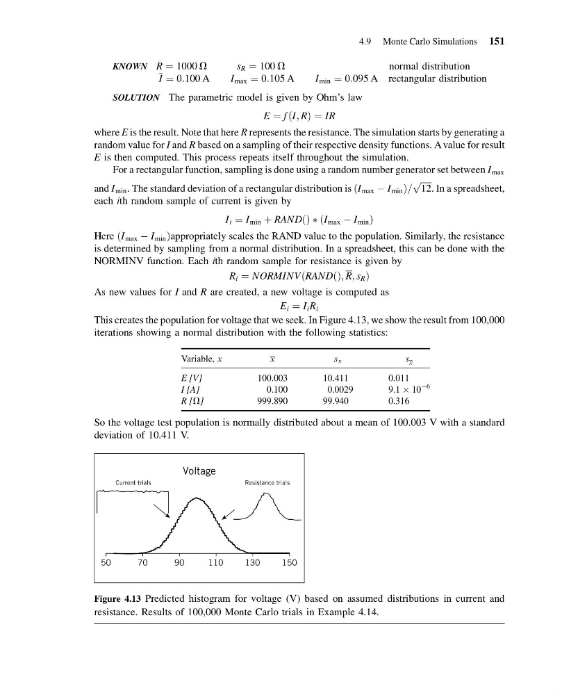
This creates the population for voltage that we seek. In Figure 4.13, we show the result from 100,000
iterations showing a normal distribution with the following statistics:
Variable, x
x
s x
s x
E [V]
100.003
10.411
0.011
I [A]
0.100
0.0029
9.1 Â 10
À6
R [V]
999.890
99.940
0.316
So the voltage test population is normally distributed about a mean of 100.003 V with a standard
deviation of 10.411 V.
50
70
90
110
130
150
Resistance trials
Current trials
Voltage
Figure 4.13 Predicted histogram for voltage (V) based on assumed distributions in current and
resistance. Results of 100,000 Monte Carlo trials in Example 4.14.
4.9 Monte Carlo Simulations 151
14:7:44 Page 151
KNOWN
R ¼ 1000 V
s R ¼ 100 V
normal distribution
I ¼ 0:100 A
I max ¼ 0:105 A
I min ¼ 0:095 A rectangular distribution
SOLUTION The parametric model is given by Ohm’s law
E ¼ f ðI; RÞ ¼ IR
where E is the result. Note that here R represents the resistance. The simulation starts by generating a
random value for I and R based on a sampling of their respective density functions. A value for result
E is then computed. This process repeats itself throughout the simulation.
For a rectangular function, sampling is done using a random number generator set between I max
and I min . The standard deviation of a rectangular distribution is ðI max À I min Þ=
ffiffiffiffiffi
12
p
. In a spreadsheet,
each ith random sample of current is given by
I i ¼ I min þ RANDðÞ Ã ðI max À I min Þ
Here ðI max À I min Þappropriately scales the RAND value to the population. Similarly, the resistance
is determined by sampling from a normal distribution. In a spreadsheet, this can be done with the
NORMINV function. Each ith random sample for resistance is given by
R i ¼ NORMINVðRANDðÞ; R; s R Þ
As new values for I and R are created, a new voltage is computed as
E i ¼ I i R i
This creates the population for voltage that we seek. In Figure 4.13, we show the result from 100,000
iterations showing a normal distribution with the following statistics:
Variable, x
x
s x
s x
E [V]
100.003
10.411
0.011
I [A]
0.100
0.0029
9.1 Â 10
À6
R [V]
999.890
99.940
0.316
So the voltage test population is normally distributed about a mean of 100.003 V with a standard
deviation of 10.411 V.
50
70
90
110
130
150
Resistance trials
Current trials
Voltage
Figure 4.13 Predicted histogram for voltage (V) based on assumed distributions in current and
resistance. Results of 100,000 Monte Carlo trials in Example 4.14.
4.9 Monte Carlo Simulations 151