

E1C04 09/14/2010
14:7:44 Page 150
4.9 MONTE CARLO SIMULATIONS
When a result is computed from the values of one or more independent random variables, the
variability in the independent variables directly affects the variability in the result. Monte Carlo
simulations provide one way to incorporate such variability into predicting the behavior of the
result. The simulation outcome is the predicted probability density function of the result, p(R), and
its associated statistics. This outcome makes it a very useful sampling method.
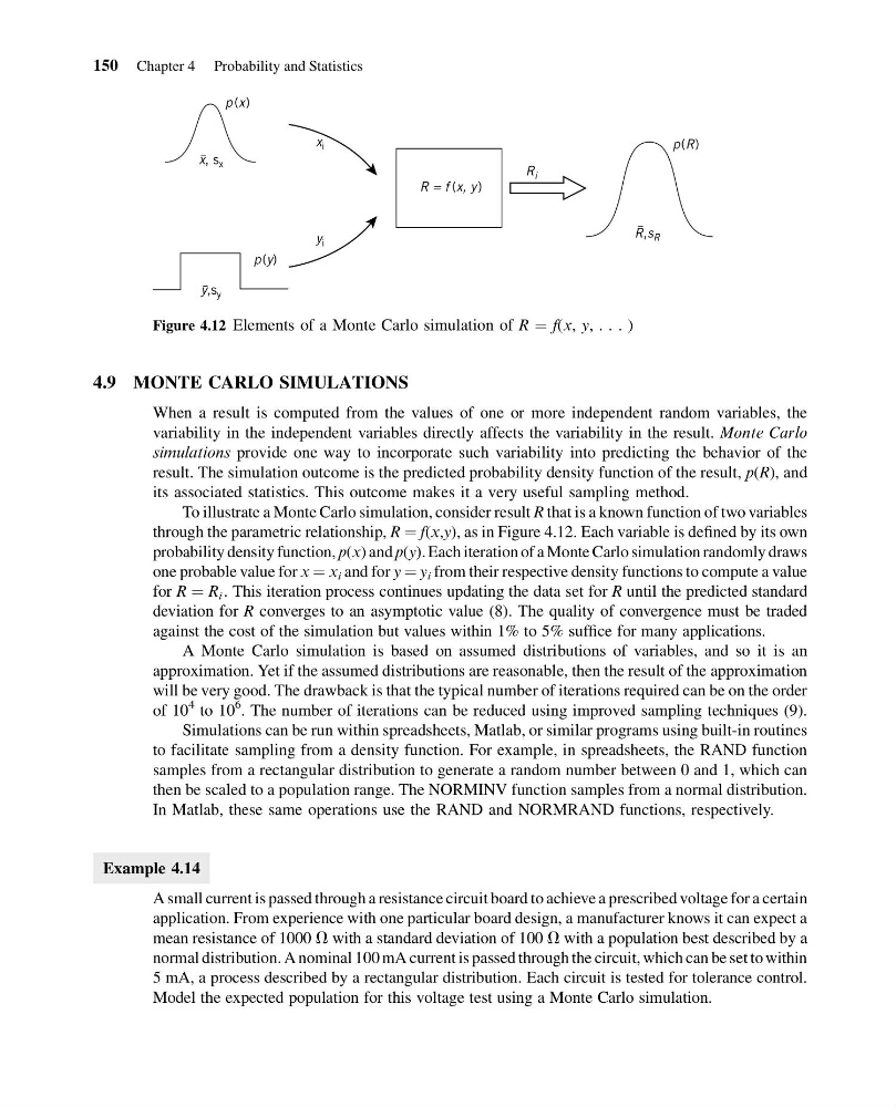
To illustrate a Monte Carlo simulation, consider result R that is a known function of two variables
through the parametric relationship, R ¼ f(x,y), as in Figure 4.12. Each variable is defined by its own
probability density function, p(x) and p(y). Each iteration of a Monte Carlo simulation randomly draws
one probable value for x ¼ x i and for y ¼ y i from their respective density functions to compute a value
for R ¼ R i . This iteration process continues updating the data set for R until the predicted standard
deviation for R converges to an asymptotic value (8). The quality of convergence must be traded
against the cost of the simulation but values within 1% to 5% suffice for many applications.
A Monte Carlo simulation is based on assumed distributions of variables, and so it is an
approximation. Yet if the assumed distributions are reasonable, then the result of the approximation
will be very good. The drawback is that the typical number of iterations required can be on the order
of 10
4 to 10
6 . The number of iterations can be reduced using improved sampling techniques (9).
Simulations can be run within spreadsheets, Matlab, or similar programs using built-in routines
to facilitate sampling from a density function. For example, in spreadsheets, the RAND function
samples from a rectangular distribution to generate a random number between 0 and 1, which can
then be scaled to a population range. The NORMINV function samples from a normal distribution.
In Matlab, these same operations use the RAND and NORMRAND functions, respectively.
Example 4.14
A small current is passed through a resistance circuit board to achieve a prescribed voltage for a certain
application. From experience with one particular board design, a manufacturer knows it can expect a
mean resistance of 1000 V with a standard deviation of 100 V with a population best described by a
normal distribution. A nominal 100 mA current is passed through the circuit, which can be set to within
5 mA, a process described by a rectangular distribution. Each circuit is tested for tolerance control.
Model the expected population for this voltage test using a Monte Carlo simulation.
p (x)
p (y)
x, s x
y,s y
R,s R
p(R)
R = f (x, y)
R i
y i
x i
Figure 4.12 Elements of a Monte Carlo simulation of R ¼ f(x, y, . . . )
150 Chapter 4 Probability and Statistics
14:7:44 Page 150
4.9 MONTE CARLO SIMULATIONS
When a result is computed from the values of one or more independent random variables, the
variability in the independent variables directly affects the variability in the result. Monte Carlo
simulations provide one way to incorporate such variability into predicting the behavior of the
result. The simulation outcome is the predicted probability density function of the result, p(R), and
its associated statistics. This outcome makes it a very useful sampling method.
To illustrate a Monte Carlo simulation, consider result R that is a known function of two variables
through the parametric relationship, R ¼ f(x,y), as in Figure 4.12. Each variable is defined by its own
probability density function, p(x) and p(y). Each iteration of a Monte Carlo simulation randomly draws
one probable value for x ¼ x i and for y ¼ y i from their respective density functions to compute a value
for R ¼ R i . This iteration process continues updating the data set for R until the predicted standard
deviation for R converges to an asymptotic value (8). The quality of convergence must be traded
against the cost of the simulation but values within 1% to 5% suffice for many applications.
A Monte Carlo simulation is based on assumed distributions of variables, and so it is an
approximation. Yet if the assumed distributions are reasonable, then the result of the approximation
will be very good. The drawback is that the typical number of iterations required can be on the order
of 10
4 to 10
6 . The number of iterations can be reduced using improved sampling techniques (9).
Simulations can be run within spreadsheets, Matlab, or similar programs using built-in routines
to facilitate sampling from a density function. For example, in spreadsheets, the RAND function
samples from a rectangular distribution to generate a random number between 0 and 1, which can
then be scaled to a population range. The NORMINV function samples from a normal distribution.
In Matlab, these same operations use the RAND and NORMRAND functions, respectively.
Example 4.14
A small current is passed through a resistance circuit board to achieve a prescribed voltage for a certain
application. From experience with one particular board design, a manufacturer knows it can expect a
mean resistance of 1000 V with a standard deviation of 100 V with a population best described by a
normal distribution. A nominal 100 mA current is passed through the circuit, which can be set to within
5 mA, a process described by a rectangular distribution. Each circuit is tested for tolerance control.
Model the expected population for this voltage test using a Monte Carlo simulation.
p (x)
p (y)
x, s x
y,s y
R,s R
p(R)
R = f (x, y)
R i
y i
x i
Figure 4.12 Elements of a Monte Carlo simulation of R ¼ f(x, y, . . . )
150 Chapter 4 Probability and Statistics