

E1C04 09/14/2010
14:7:40 Page 121
of x into K small intervals. Let the number of times, n j , that a measured value assumes a value
within an interval defined by x À dx x x þ dx be plotted on the ordinate. The resulting plot of
n j versus x is called a histogram of the variable (1). The histogram is just another way of viewing
both the tendency and the probability density of a variable. The ordinate can be nondimensionalized as f j ¼ n j /N, converting the histogram into a frequency distribution. For small N, the interval
number K should be conveniently chosen with a good rule that n j ! 5 for at least one interval. A
correlation for an estimate for the number of intervals K is derived from the suggestions in Bendat
and Piersol (2) as
K ¼ 1:87ðN À 1Þ
0:40 þ 1
ð4:2Þ
As N becomes very large, a value of K % N
1/2 works reasonably well (1, 2). The concept of the
histogram is illustrated in Example 4.1.
Example 4.1
Construct a histogram and frequency distribution for the data in Table 4.1.
KNOWN Data of Table 4.1
N ¼ 20
ASSUMPTIONS Fixed operating conditions
FIND Histogram and frequency distribution
SOLUTION To develop the histogram, compute a reasonable number of intervals for this data
set. For N ¼ 20, a convenient estimate of K is found from Equation 4.2 to be
K ¼ 1:87ðN À 1Þ
0:40 þ 1 ¼ 7
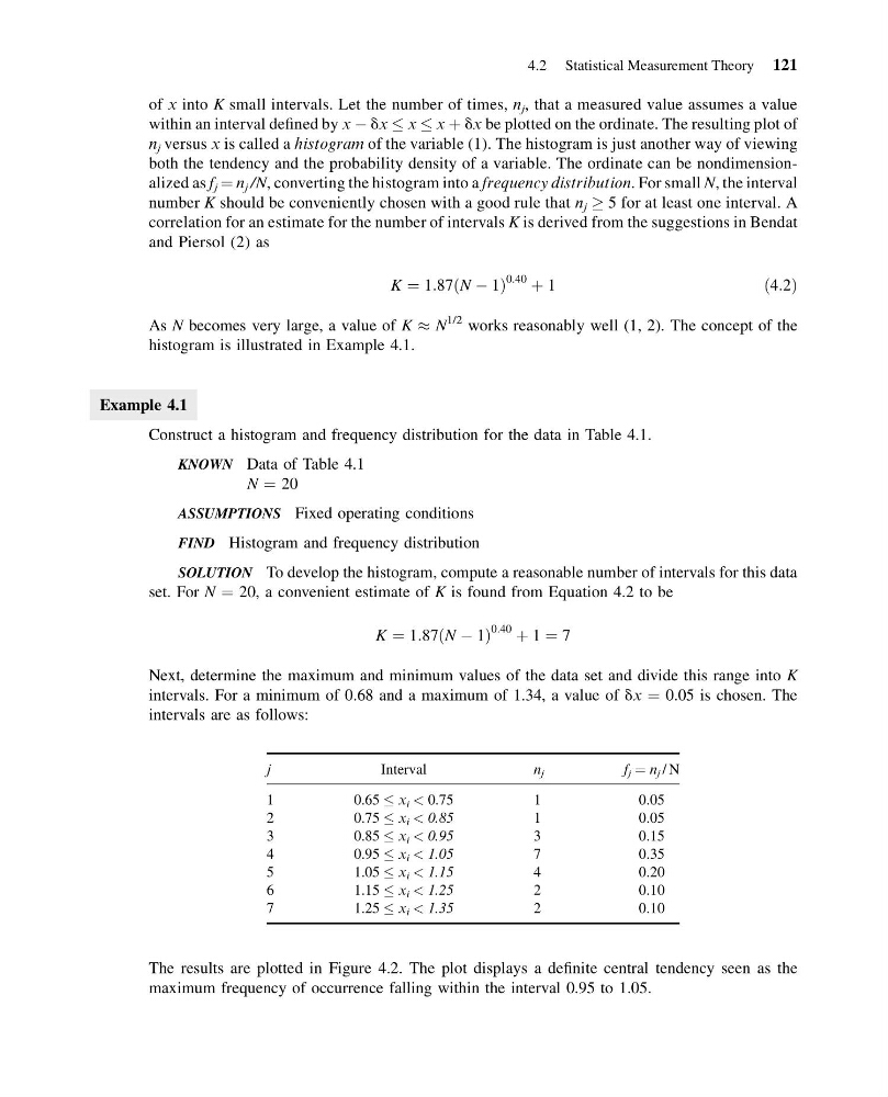
Next, determine the maximum and minimum values of the data set and divide this range into K
intervals. For a minimum of 0.68 and a maximum of 1.34, a value of dx ¼ 0.05 is chosen. The
intervals are as follows:
j
Interval
n j
f j ¼ n j / N
1
0.65 x i < 0.75
1
0.05
2
0.75 x i < 0.85
1
0.05
3
0.85 x i < 0.95
3
0.15
4
0.95 x i < 1.05
7
0.35
5
1.05 x i < 1.15
4
0.20
6
1.15 x i < 1.25
2
0.10
7
1.25 x i < 1.35
2
0.10
The results are plotted in Figure 4.2. The plot displays a definite central tendency seen as the
maximum frequency of occurrence falling within the interval 0.95 to 1.05.
4.2 Statistical Measurement Theory 121
14:7:40 Page 121
of x into K small intervals. Let the number of times, n j , that a measured value assumes a value
within an interval defined by x À dx x x þ dx be plotted on the ordinate. The resulting plot of
n j versus x is called a histogram of the variable (1). The histogram is just another way of viewing
both the tendency and the probability density of a variable. The ordinate can be nondimensionalized as f j ¼ n j /N, converting the histogram into a frequency distribution. For small N, the interval
number K should be conveniently chosen with a good rule that n j ! 5 for at least one interval. A
correlation for an estimate for the number of intervals K is derived from the suggestions in Bendat
and Piersol (2) as
K ¼ 1:87ðN À 1Þ
0:40 þ 1
ð4:2Þ
As N becomes very large, a value of K % N
1/2 works reasonably well (1, 2). The concept of the
histogram is illustrated in Example 4.1.
Example 4.1
Construct a histogram and frequency distribution for the data in Table 4.1.
KNOWN Data of Table 4.1
N ¼ 20
ASSUMPTIONS Fixed operating conditions
FIND Histogram and frequency distribution
SOLUTION To develop the histogram, compute a reasonable number of intervals for this data
set. For N ¼ 20, a convenient estimate of K is found from Equation 4.2 to be
K ¼ 1:87ðN À 1Þ
0:40 þ 1 ¼ 7
Next, determine the maximum and minimum values of the data set and divide this range into K
intervals. For a minimum of 0.68 and a maximum of 1.34, a value of dx ¼ 0.05 is chosen. The
intervals are as follows:
j
Interval
n j
f j ¼ n j / N
1
0.65 x i < 0.75
1
0.05
2
0.75 x i < 0.85
1
0.05
3
0.85 x i < 0.95
3
0.15
4
0.95 x i < 1.05
7
0.35
5
1.05 x i < 1.15
4
0.20
6
1.15 x i < 1.25
2
0.10
7
1.25 x i < 1.35
2
0.10
The results are plotted in Figure 4.2. The plot displays a definite central tendency seen as the
maximum frequency of occurrence falling within the interval 0.95 to 1.05.
4.2 Statistical Measurement Theory 121