

E1C04 09/14/2010
14:7:40 Page 120
Probability Density Functions
Random scatter of the measured data occurs regardless of the care taken to obtain the set from
independent measurements under identical conditions. As such, the measured variable behaves as a
random variable. A continuous random variable is one that is continuous in time or space, such as
the value of a motor’s speed. A discrete random variable is one that is composed of discrete values,
such as the values of the diameters of the bearings mentioned in Section 4.1. During repeated
measurements of a variable, each data point may tend to assume one preferred value or lie within
some interval about this value more often than not, when all the data are compared. This tendency
toward one central value about which all the other values are scattered is known as a central
tendency of a random variable.
3 Probability deals with the concept that certain values of a variable
may be measured more frequently relative to other values.
The central value and those values scattered about it can be determined from the probability
density of the measured variable. The frequency with which the measured variable assumes a
particular value or interval of values is described by its probability density. Consider a sample of x
shown in Table 4.1, which consists of N individual measurements, x i , where i ¼ 2, . . . , N, each
measurement taken at random but under identical test operating conditions. The measured values of
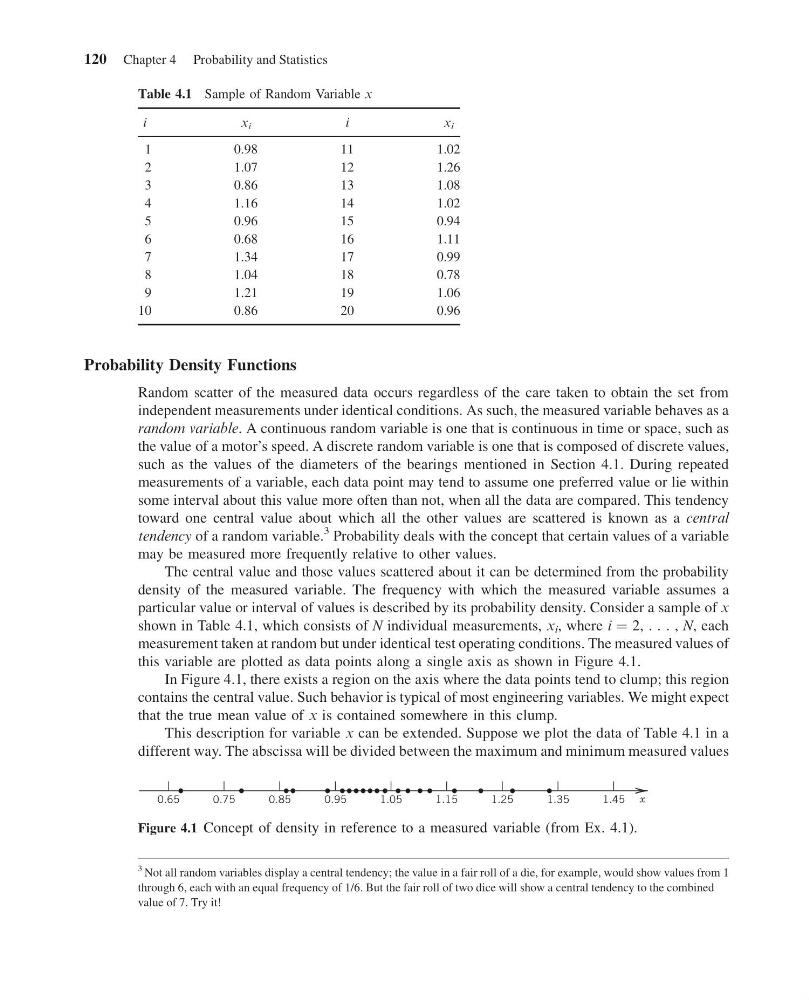
this variable are plotted as data points along a single axis as shown in Figure 4.1.
In Figure 4.1, there exists a region on the axis where the data points tend to clump; this region
contains the central value. Such behavior is typical of most engineering variables. We might expect
that the true mean value of x is contained somewhere in this clump.
This description for variable x can be extended. Suppose we plot the data of Table 4.1 in a
different way. The abscissa will be divided between the maximum and minimum measured values
Table 4.1 Sample of Random Variable x
i
x i
i
x i
1
0.98
11
1.02
2
1.07
12
1.26
3
0.86
13
1.08
4
1.16
14
1.02
5
0.96
15
0.94
6
0.68
16
1.11
7
1.34
17
0.99
8
1.04
18
0.78
9
1.21
19
1.06
10
0.86
20
0.96
x
1.45
1.35
1.25
1.15
1.05
0.95
0.85
0.75
0.65
Figure 4.1 Concept of density in reference to a measured variable (from Ex. 4.1).
3 Not all random variables display a central tendency; the value in a fair roll of a die, for example, would show values from 1
through 6, each with an equal frequency of 1/6. But the fair roll of two dice will show a central tendency to the combined
value of 7. Try it!
120 Chapter 4 Probability and Statistics
14:7:40 Page 120
Probability Density Functions
Random scatter of the measured data occurs regardless of the care taken to obtain the set from
independent measurements under identical conditions. As such, the measured variable behaves as a
random variable. A continuous random variable is one that is continuous in time or space, such as
the value of a motor’s speed. A discrete random variable is one that is composed of discrete values,
such as the values of the diameters of the bearings mentioned in Section 4.1. During repeated
measurements of a variable, each data point may tend to assume one preferred value or lie within
some interval about this value more often than not, when all the data are compared. This tendency
toward one central value about which all the other values are scattered is known as a central
tendency of a random variable.
3 Probability deals with the concept that certain values of a variable
may be measured more frequently relative to other values.
The central value and those values scattered about it can be determined from the probability
density of the measured variable. The frequency with which the measured variable assumes a
particular value or interval of values is described by its probability density. Consider a sample of x
shown in Table 4.1, which consists of N individual measurements, x i , where i ¼ 2, . . . , N, each
measurement taken at random but under identical test operating conditions. The measured values of
this variable are plotted as data points along a single axis as shown in Figure 4.1.
In Figure 4.1, there exists a region on the axis where the data points tend to clump; this region
contains the central value. Such behavior is typical of most engineering variables. We might expect
that the true mean value of x is contained somewhere in this clump.
This description for variable x can be extended. Suppose we plot the data of Table 4.1 in a
different way. The abscissa will be divided between the maximum and minimum measured values
Table 4.1 Sample of Random Variable x
i
x i
i
x i
1
0.98
11
1.02
2
1.07
12
1.26
3
0.86
13
1.08
4
1.16
14
1.02
5
0.96
15
0.94
6
0.68
16
1.11
7
1.34
17
0.99
8
1.04
18
0.78
9
1.21
19
1.06
10
0.86
20
0.96
x
1.45
1.35
1.25
1.15
1.05
0.95
0.85
0.75
0.65
Figure 4.1 Concept of density in reference to a measured variable (from Ex. 4.1).
3 Not all random variables display a central tendency; the value in a fair roll of a die, for example, would show values from 1
through 6, each with an equal frequency of 1/6. But the fair roll of two dice will show a central tendency to the combined
value of 7. Try it!
120 Chapter 4 Probability and Statistics