

E1C04 09/14/2010
14:7:40 Page 122
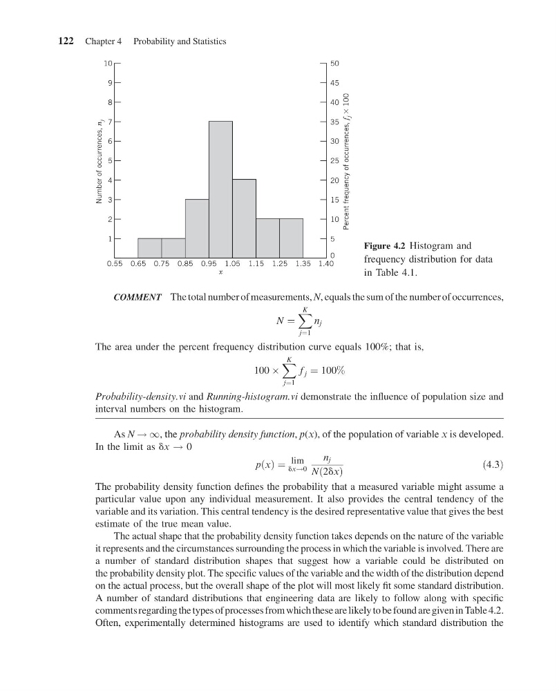
COMMENT The total number of measurements, N, equals the sum of the number of occurrences,
N ¼
X K
j¼1
n j
The area under the percent frequency distribution curve equals 100%; that is,
100 Â
X K
j¼1
f j ¼ 100%
Probability-density.vi and Running-histogram.vi demonstrate the influence of population size and
interval numbers on the histogram.
As N ! 1, the probability density function, p(x), of the population of variable x is developed.
In the limit as dx ! 0
p x
ð Þ ¼ lim
dx!0
n j
N 2dx
ð
Þ
ð4:3Þ
The probability density function defines the probability that a measured variable might assume a
particular value upon any individual measurement. It also provides the central tendency of the
variable and its variation. This central tendency is the desired representative value that gives the best
estimate of the true mean value.
The actual shape that the probability density function takes depends on the nature of the variable
it represents and the circumstances surrounding the process in which the variable is involved. There are
a number of standard distribution shapes that suggest how a variable could be distributed on
the probability density plot. The specific values of the variable and the width of the distribution depend
on the actual process, but the overall shape of the plot will most likely fit some standard distribution.
A number of standard distributions that engineering data are likely to follow along with specific
comments regarding the types of processes from which these are likely to be found are given in Table 4.2.
Often, experimentally determined histograms are used to identify which standard distribution the
0.55 0.65 0.75 0.85 0.95 1.05 1.15 1.25 1.35 1.40
x
Number of occurrences,
n
j
1
2
3
4
5
6
7
8
9
10
Percent frequency of occurrences,
f
j
100
5
0
10
15
20
25
30
35
40
45
50
Figure 4.2 Histogram and
frequency distribution for data
in Table 4.1.
122 Chapter 4 Probability and Statistics
14:7:40 Page 122
COMMENT The total number of measurements, N, equals the sum of the number of occurrences,
N ¼
X K
j¼1
n j
The area under the percent frequency distribution curve equals 100%; that is,
100 Â
X K
j¼1
f j ¼ 100%
Probability-density.vi and Running-histogram.vi demonstrate the influence of population size and
interval numbers on the histogram.
As N ! 1, the probability density function, p(x), of the population of variable x is developed.
In the limit as dx ! 0
p x
ð Þ ¼ lim
dx!0
n j
N 2dx
ð
Þ
ð4:3Þ
The probability density function defines the probability that a measured variable might assume a
particular value upon any individual measurement. It also provides the central tendency of the
variable and its variation. This central tendency is the desired representative value that gives the best
estimate of the true mean value.
The actual shape that the probability density function takes depends on the nature of the variable
it represents and the circumstances surrounding the process in which the variable is involved. There are
a number of standard distribution shapes that suggest how a variable could be distributed on
the probability density plot. The specific values of the variable and the width of the distribution depend
on the actual process, but the overall shape of the plot will most likely fit some standard distribution.
A number of standard distributions that engineering data are likely to follow along with specific
comments regarding the types of processes from which these are likely to be found are given in Table 4.2.
Often, experimentally determined histograms are used to identify which standard distribution the
0.55 0.65 0.75 0.85 0.95 1.05 1.15 1.25 1.35 1.40
x
Number of occurrences,
n
j
1
2
3
4
5
6
7
8
9
10
Percent frequency of occurrences,
f
j
100
5
0
10
15
20
25
30
35
40
45
50
Figure 4.2 Histogram and
frequency distribution for data
in Table 4.1.
122 Chapter 4 Probability and Statistics