

670
G Hamiltonian Mechanics
We can see from these two results that there will be 2N integration constants,
corresponding to the set of values {q k (0), p k (0)} at some time t 0 = 0.
-space: for a system consisting of N molecules, each of which has s degrees of
freedom, we have a total of 2sN generalized coordinates (q k , p k ). We define a 2N -
dimensional Cartesian space whose axes are the {q k , p k } variables, so that the state
of an N-molecule system at any given instant of time, specified by the coordinates
(q 1 , · · · , q N , p 1 , · · · , p N ) is represented by a single point in this 2N-dimensional
Cartesian space. This Cartesian space is called the phase space of the system or,
for short, -space. If we add time explicitly to our considerations, the augmented
(2N + 1)-dimensional Cartesian space is called the -space.
G.3.3 Hamilton’s Principle and Generating Functions
It is often useful to be able to transform from one set of coordinates {q i } to a new
set of coordinates {Q i } in which the equations of motion can be simplified and
a clean solution obtained. Of course, the new coordinates Q will be functions of
the old coordinates q and t: i.e., Q i = Q i (q, t). When the new coordinates Q are
functions only of the coordinates q and t, such a transformation is called a point
transformation. However, in Hamiltonian mechanics the generalized momenta are
also independent variables on the same level as the generalized coordinates, so that
we must broaden our definition of the transformation to
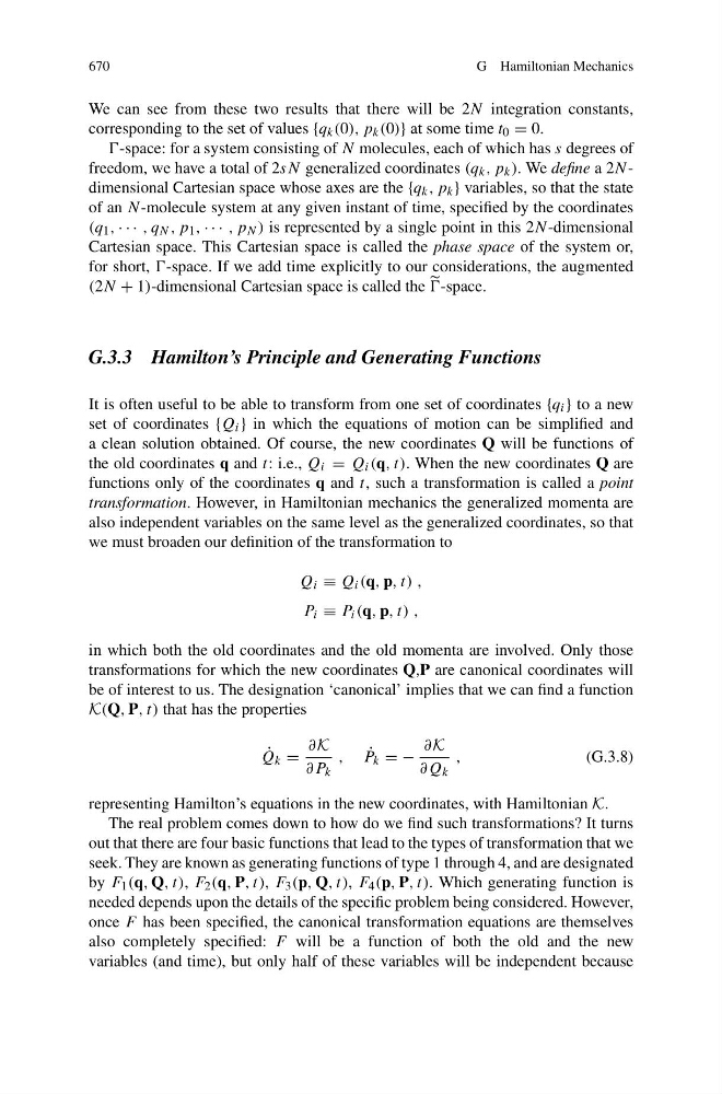
Q i ≡ Q i (q, p, t) ,
P i ≡ P i (q, p, t) ,
in which both the old coordinates and the old momenta are involved. Only those
transformations for which the new coordinates Q,P are canonical coordinates will
be of interest to us. The designation ‘canonical’ implies that we can find a function
K(Q, P, t) that has the properties
˙
Q k =
∂K
∂P k
,
˙
P k = −
∂K
∂Q k
,
(G.3.8)
representing Hamilton’s equations in the new coordinates, with Hamiltonian K.
The real problem comes down to how do we find such transformations? It turns
out that there are four basic functions that lead to the types of transformation that we
seek. They are known as generating functions of type 1 through 4, and are designated
by F 1 (q, Q, t), F 2 (q, P, t), F 3 (p, Q, t), F 4 (p, P, t). Which generating function is
needed depends upon the details of the specific problem being considered. However,
once F has been specified, the canonical transformation equations are themselves
also completely specified: F will be a function of both the old and the new
variables (and time), but only half of these variables will be independent because