G.3 Hamilton’s Equations
671
of the transformation equations (G.3.8). The origin of these generating functions for
canonical transformations lies in Hamilton’s Principle.
Hamilton’s principle states that the motion of a system from time t 1 to time t 2 is
such that the line integral I =
t 2
t 1
L dt, with L ≡ T − V , is an extremum (normally
a minimum) for the path of motion. In other words, any variation of the line integral
I for fixed t 1 and t 2 must vanish: this requirement is expressed as
δI = δ
t 2
t 1
L(q, ˙
q, t) dt = 0 .
The expression for δI is known as a variational principle, and comes out of a
field of mathematics known as the calculus of variations, highlighted briefly in
Appendix B. Hamilton’s Principle must apply both to the old set of generalized
coordinates {q, p, t} with its corresponding Hamiltonian function H, and to the new
set of generalized coordinates {Q, P, t} and its corresponding Hamiltonian K. Thus,
we have two conditions,
δ
t 2
t 1
i
P i ˙
Q i − K(Q, P, t)
dt = 0
(G.3.9)
and
δ
t 2
t 1
i
p i ˙
q i − H(q, p, t)
dt = 0
(G.3.10)
that must be satisfied simultaneously. This means that the two integrands can differ
at most by a total time derivative of an arbitrary function F (t) that is constrained so
that
t 2
t 1
dF
dt
dt = F (t 2 ) − F (t 1 ) ,
which automatically vanishes because the variation vanishes by construction at the
end-points of the integral.
The integrands (G.3.9) and (G.3.10) can be connected by the relation
k
p k ˙
q k − H =
k
P k ˙
Q k − K +
d
dt
F 1 (q, Q, t) ,
(G.3.11)
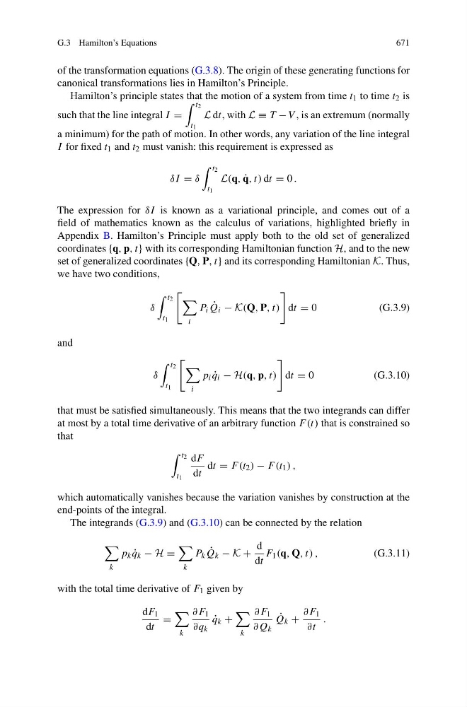
with the total time derivative of F 1 given by
dF 1
dt
=
k
∂F 1
∂q k
˙
q k +
k
∂F 1
∂Q k
˙
Q k +
∂F 1
∂t
.