G.2 Lagrangian Formulation
665
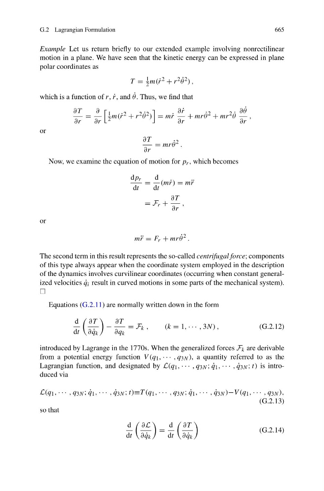
Example Let us return briefly to our extended example involving nonrectilinear
motion in a plane. We have seen that the kinetic energy can be expressed in plane
polar coordinates as
T =
1
2 m(˙ r 2 + r 2 ˙
θ 2 ) ,
which is a function of r, ˙
r, and ˙
θ . Thus, we find that
∂T
∂r
=
∂
∂r
1
2 m(˙ r 2 + r 2 ˙
θ 2 )
= m˙ r
∂ ˙
r
∂r
+ mr ˙
θ
2
+ mr
2 ˙
θ
∂ ˙
θ
∂r
,
or
∂T
∂r
= mr ˙
θ
2 .
Now, we examine the equation of motion for p r , which becomes
dp r
dt
=
d
dt
(m˙ r) = m¨ r
= F r +
∂T
∂r
,
or
m¨ r = F r + mr ˙
θ
2 .
The second term in this result represents the so-called centrifugal force; components
of this type always appear when the coordinate system employed in the description
of the dynamics involves curvilinear coordinates (occurring when constant generalized velocities ˙
q i result in curved motions in some parts of the mechanical system).
Equations (G.2.11) are normally written down in the form
d
dt
∂T
∂ ˙
q k
−
∂T
∂q k
= F k ,
(k = 1, · · · , 3N) ,
(G.2.12)
introduced by Lagrange in the 1770s. When the generalized forces F k are derivable
from a potential energy function V (q 1 , · · · , q 3N ), a quantity referred to as the
Lagrangian function, and designated by L(q 1 , · · · , q 3N ; ˙
q 1 , · · · , ˙
q 3N ; t) is introduced via
L(q 1 , · · · , q 3N ; ˙
q 1 , · · · , ˙
q 3N ; t)≡T (q 1 , · · · , q 3N ; ˙
q 1 , · · · , ˙
q 3N )−V (q 1 , · · · , q 3N ),
(G.2.13)
so that
d
dt
∂L
∂ ˙
q k
=
d
dt
∂T
∂ ˙
q k
(G.2.14)