

24
1 Basic Background Material
v = = v − −v = =v − −v = 0 .
We know that there is scatter of the individual measurements about the mean value,
so that v does not provide for us a measure in the mean of how much scatter
there is in the set of measurements. Obviously, in order to measure the scatter, we
shall need a quantity that is always positive; such a quantity is given by ((v) 2 . Let
us now calculate the mean of this quantity:
((v)
2
= =v
2
− −v
2 .
(1.4.19)
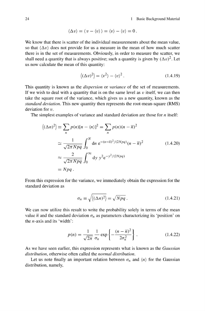
This quantity is known as the dispersion or variance of the set of measurements.
If we wish to deal with a quantity that is on the same level as v itself, we can then
take the square root of the variance, which gives us a new quantity, known as the
standard deviation. This new quantity then represents the root-mean-square (RMS)
deviation for v.
The simplest examples of variance and standard deviation are those for n itself:
((n)
2
≡
n
p(n)[n − −n]
2
=
n
p(n)(n − n)
2
1
√
2πNpq
N
0
dn e
−(n−n) 2 /(2Npq) (n − n)
2
(1.4.20)
≈
2
√
2πNpq
∞
0
dy y
2 e
−y 2 /(2Npq)
= Npq .
From this expression for the variance, we immediately obtain the expression for the
standard deviation as
σ n ≡
((n) 2
=
Npq .
(1.4.21)
We can now utilize this result to write the probability solely in terms of the mean
value n and the standard deviation σ n as parameters characterizing its ‘position’ on
the n-axis and its ‘width’:
p(n) =
1
√
2π
1
σ n
exp
−
(n − n) 2
2σ 2
n
.
(1.4.22)
As we have seen earlier, this expression represents what is known as the Gaussian
distribution, otherwise often called the normal distribution.
Let us note finally an important relation between σ n and n for the Gaussian
distribution, namely,
1 Basic Background Material
v = = v − −v = =v − −v = 0 .
We know that there is scatter of the individual measurements about the mean value,
so that v does not provide for us a measure in the mean of how much scatter
there is in the set of measurements. Obviously, in order to measure the scatter, we
shall need a quantity that is always positive; such a quantity is given by ((v) 2 . Let
us now calculate the mean of this quantity:
((v)
2
= =v
2
− −v
2 .
(1.4.19)
This quantity is known as the dispersion or variance of the set of measurements.
If we wish to deal with a quantity that is on the same level as v itself, we can then
take the square root of the variance, which gives us a new quantity, known as the
standard deviation. This new quantity then represents the root-mean-square (RMS)
deviation for v.
The simplest examples of variance and standard deviation are those for n itself:
((n)
2
≡
n
p(n)[n − −n]
2
=
n
p(n)(n − n)
2
1
√
2πNpq
N
0
dn e
−(n−n) 2 /(2Npq) (n − n)
2
(1.4.20)
≈
2
√
2πNpq
∞
0
dy y
2 e
−y 2 /(2Npq)
= Npq .
From this expression for the variance, we immediately obtain the expression for the
standard deviation as
σ n ≡
((n) 2
=
Npq .
(1.4.21)
We can now utilize this result to write the probability solely in terms of the mean
value n and the standard deviation σ n as parameters characterizing its ‘position’ on
the n-axis and its ‘width’:
p(n) =
1
√
2π
1
σ n
exp
−
(n − n) 2
2σ 2
n
.
(1.4.22)
As we have seen earlier, this expression represents what is known as the Gaussian
distribution, otherwise often called the normal distribution.
Let us note finally an important relation between σ n and n for the Gaussian
distribution, namely,