

1.4 Statistical Ensembles
23
so that, using Eq. (1.4.14) in the integral form of the normalization condition, we
have that
p(N, n)
N
0
dn e
−(n−n) 2 /(2Npq)
= 1 .
Evaluation of the integral gives us a final expression for the Gaussian probability
distribution, namely
p(N, n) =
1
√
2πNpq
e
−(n−n) 2 /(2Npq) ,
(1.4.17)
in which N, n are both very large.
We can now use this expression for p(N, n) to evaluate the average value of n
itself in the following way:
n ≡
n
np(N, n)
1
√
2πNpq
N
0
dn ne
−(n−n) 2 /(2Npq) ,
from which we obtain the result
n = n .
(1.4.18)
Hence, for this special distribution, the average value of n is also its most probable
value.
1.4.2 Variance and Standard Deviation
Let us consider a set of N ‘measurements’ of a quantity v compared with its
mean value v. The deviation of an individual ‘measurement’ from the mean value
is expressed by v = v − −v . The set of measurements is, by construction,
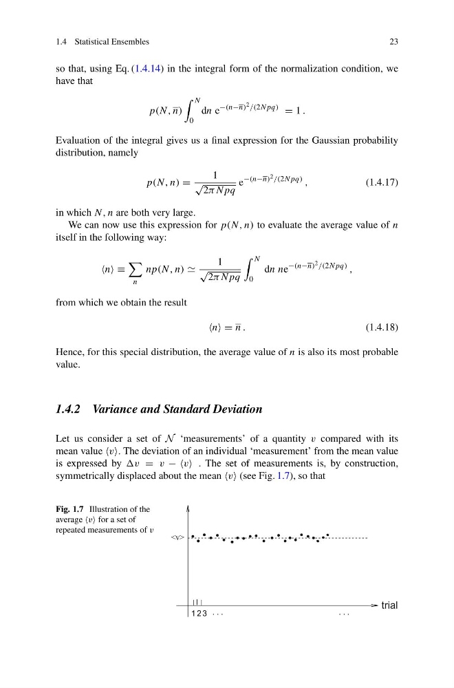
symmetrically displaced about the mean v (see Fig. 1.7), so that
Fig. 1.7 Illustration of the
average v for a set of
repeated measurements of v
trial
1 2 3 . . .
. . .
23
so that, using Eq. (1.4.14) in the integral form of the normalization condition, we
have that
p(N, n)
N
0
dn e
−(n−n) 2 /(2Npq)
= 1 .
Evaluation of the integral gives us a final expression for the Gaussian probability
distribution, namely
p(N, n) =
1
√
2πNpq
e
−(n−n) 2 /(2Npq) ,
(1.4.17)
in which N, n are both very large.
We can now use this expression for p(N, n) to evaluate the average value of n
itself in the following way:
n ≡
n
np(N, n)
1
√
2πNpq
N
0
dn ne
−(n−n) 2 /(2Npq) ,
from which we obtain the result
n = n .
(1.4.18)
Hence, for this special distribution, the average value of n is also its most probable
value.
1.4.2 Variance and Standard Deviation
Let us consider a set of N ‘measurements’ of a quantity v compared with its
mean value v. The deviation of an individual ‘measurement’ from the mean value
is expressed by v = v − −v . The set of measurements is, by construction,
symmetrically displaced about the mean v (see Fig. 1.7), so that
Fig. 1.7 Illustration of the
average v for a set of
repeated measurements of v
trial
1 2 3 . . .
. . .