

22
1 Basic Background Material
N − n
n
p
q
= 1 ,
(1.4.9)
or
Np = n(p + q) ≡ n .
(1.4.10)
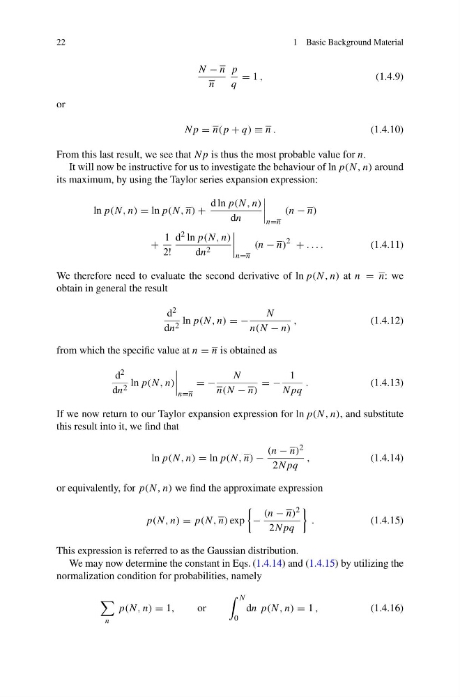
From this last result, we see that Np is thus the most probable value for n.
It will now be instructive for us to investigate the behaviour of ln p(N, n) around
its maximum, by using the Taylor series expansion expression:
ln p(N, n) = ln p(N, n) +
d ln p(N, n)
dn
n=n
(n − n)
+
1
2!
d 2 ln p(N, n)
dn 2
n=n
(n − n)
2
+ . . . .
(1.4.11)
We therefore need to evaluate the second derivative of ln p(N, n) at n = n: we
obtain in general the result
d 2
dn 2 ln p(N, n) = −
N
n(N − n)
,
(1.4.12)
from which the specific value at n = n is obtained as
d 2
dn 2 ln p(N, n)
n=n
= −
N
n(N − n)
= −
1
Npq
.
(1.4.13)
If we now return to our Taylor expansion expression for ln p(N, n), and substitute
this result into it, we find that
ln p(N, n) = ln p(N, n) −
(n − n) 2
2Npq
,
(1.4.14)
or equivalently, for p(N, n) we find the approximate expression
p(N, n) = p(N, n) exp
−
(n − n) 2
2Npq
.
(1.4.15)
This expression is referred to as the Gaussian distribution.
We may now determine the constant in Eqs. (1.4.14) and (1.4.15) by utilizing the
normalization condition for probabilities, namely
n
p(N, n) = 1,
or
N
0
dn p(N, n) = 1 ,
(1.4.16)
1 Basic Background Material
N − n
n
p
q
= 1 ,
(1.4.9)
or
Np = n(p + q) ≡ n .
(1.4.10)
From this last result, we see that Np is thus the most probable value for n.
It will now be instructive for us to investigate the behaviour of ln p(N, n) around
its maximum, by using the Taylor series expansion expression:
ln p(N, n) = ln p(N, n) +
d ln p(N, n)
dn
n=n
(n − n)
+
1
2!
d 2 ln p(N, n)
dn 2
n=n
(n − n)
2
+ . . . .
(1.4.11)
We therefore need to evaluate the second derivative of ln p(N, n) at n = n: we
obtain in general the result
d 2
dn 2 ln p(N, n) = −
N
n(N − n)
,
(1.4.12)
from which the specific value at n = n is obtained as
d 2
dn 2 ln p(N, n)
n=n
= −
N
n(N − n)
= −
1
Npq
.
(1.4.13)
If we now return to our Taylor expansion expression for ln p(N, n), and substitute
this result into it, we find that
ln p(N, n) = ln p(N, n) −
(n − n) 2
2Npq
,
(1.4.14)
or equivalently, for p(N, n) we find the approximate expression
p(N, n) = p(N, n) exp
−
(n − n) 2
2Npq
.
(1.4.15)
This expression is referred to as the Gaussian distribution.
We may now determine the constant in Eqs. (1.4.14) and (1.4.15) by utilizing the
normalization condition for probabilities, namely
n
p(N, n) = 1,
or
N
0
dn p(N, n) = 1 ,
(1.4.16)