

1.4 Statistical Ensembles
19
system is given by knowing each value {v 1 , v 2 , . . . , v M } of v and the corresponding
probabilities of occurrence {p 1 , p 2 , . . . , p M }. If there are N similar systems in the
ensemble, then v has the value v r in N r = N p r of them. With so many possibilities
in principle, we should be willing to settle for a little less detail; that is, we might
be interested in first instance only in the average value of the variable (other names
for this quantity are: mean value, ensemble average) defined by
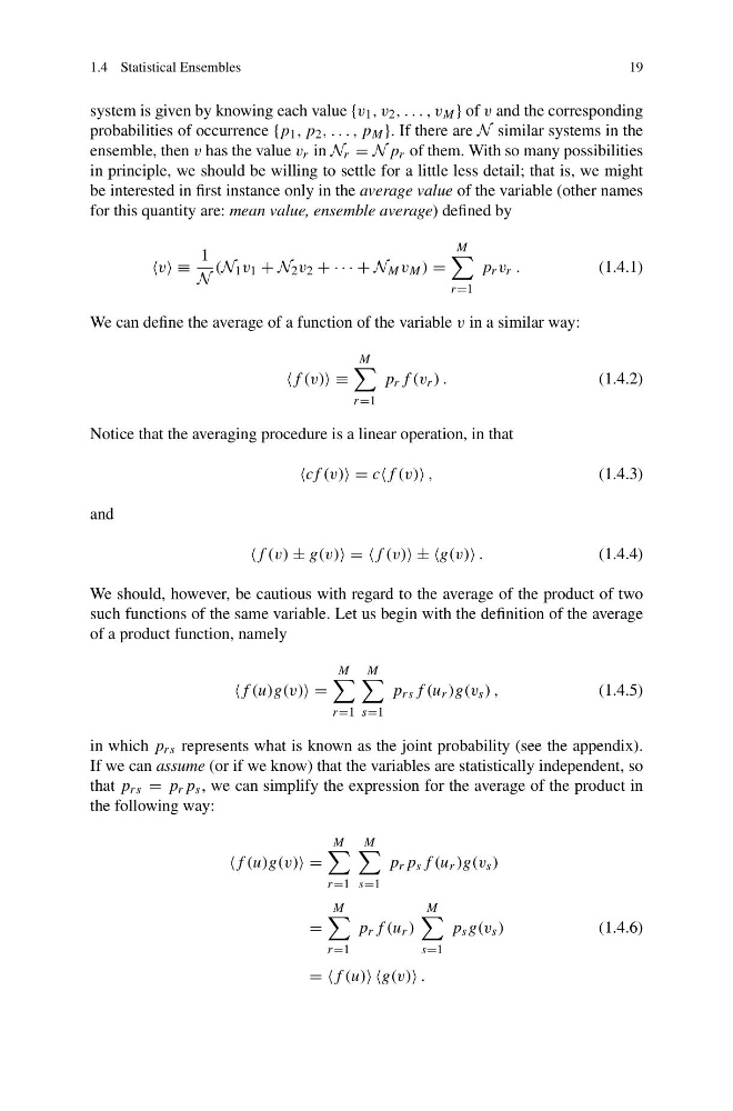
v ≡
1
N
(N 1 v 1 + N 2 v 2 + · · · + N M v M ) =
M
r=1
p r v r .
(1.4.1)
We can define the average of a function of the variable v in a similar way:
f (v) ≡
M
r=1
p r f (v r ) .
(1.4.2)
Notice that the averaging procedure is a linear operation, in that
cf (v) = cf (v) ,
(1.4.3)
and
f (v) ± g(v) = =f (v) ± ±g(v) .
(1.4.4)
We should, however, be cautious with regard to the average of the product of two
such functions of the same variable. Let us begin with the definition of the average
of a product function, namely
f (u)g(v) =
M
r=1
M
s=1
p rs f (u r )g(v s ) ,
(1.4.5)
in which p rs represents what is known as the joint probability (see the appendix).
If we can assume (or if we know) that the variables are statistically independent, so
that p rs = p r p s , we can simplify the expression for the average of the product in
the following way:
f (u)g(v) =
M
r=1
M
s=1
p r p s f (u r )g(v s )
=
M
r=1
p r f (u r )
M
s=1
p s g(v s )
(1.4.6)
= =f (u) g(v) .
19
system is given by knowing each value {v 1 , v 2 , . . . , v M } of v and the corresponding
probabilities of occurrence {p 1 , p 2 , . . . , p M }. If there are N similar systems in the
ensemble, then v has the value v r in N r = N p r of them. With so many possibilities
in principle, we should be willing to settle for a little less detail; that is, we might
be interested in first instance only in the average value of the variable (other names
for this quantity are: mean value, ensemble average) defined by
v ≡
1
N
(N 1 v 1 + N 2 v 2 + · · · + N M v M ) =
M
r=1
p r v r .
(1.4.1)
We can define the average of a function of the variable v in a similar way:
f (v) ≡
M
r=1
p r f (v r ) .
(1.4.2)
Notice that the averaging procedure is a linear operation, in that
cf (v) = cf (v) ,
(1.4.3)
and
f (v) ± g(v) = =f (v) ± ±g(v) .
(1.4.4)
We should, however, be cautious with regard to the average of the product of two
such functions of the same variable. Let us begin with the definition of the average
of a product function, namely
f (u)g(v) =
M
r=1
M
s=1
p rs f (u r )g(v s ) ,
(1.4.5)
in which p rs represents what is known as the joint probability (see the appendix).
If we can assume (or if we know) that the variables are statistically independent, so
that p rs = p r p s , we can simplify the expression for the average of the product in
the following way:
f (u)g(v) =
M
r=1
M
s=1
p r p s f (u r )g(v s )
=
M
r=1
p r f (u r )
M
s=1
p s g(v s )
(1.4.6)
= =f (u) g(v) .