

198
4 Mean Values and Thermodynamics
and
t N ∗ = Z N ∗ λ
N ∗ .
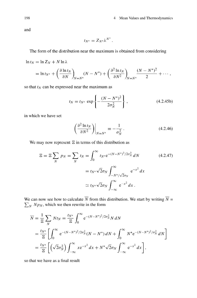
The form of the distribution near the maximum is obtained from considering
ln t N = ln Z N + N ln λ
= ln t N ∗ +
∂ ln t N
∂N
N =N ∗
(N − N
∗ ) +
∂ 2 ln t N
∂N 2
N =N ∗
(N − N ∗ ) 2
2
+ · · · ,
so that t N can be expressed near the maximum as
t N = t N ∗ exp
−
(N − N ∗ ) 2
2σ 2
N
,
(4.2.45b)
in which we have set
∂ 2 ln t N
∂N 2
N =N ∗
≡ −
1
σ 2
N
.
(4.2.46)
We may now represent in terms of this distribution as
=
N
p N =
N
t N =
∞
0
t N ∗ e
−(N −N ∗ ) 2 /2σ 2
N dN
(4.2.47)
= t N ∗
√
2σ N
∞
−N ∗ /
√
2σ N
e
−x 2 dx
t N ∗
√
2σ N
∞
−∞
e
−x 2 dx .
We can now see how to calculate N from this distribution. We start by writing N =
N Np N , which we then rewrite in the form
N =
1
N
Nt N =
t N ∗
∞
0
e
−(N −N ∗ ) 2 /2σ 2
N N dN
=
t N ∗
∞
0
e
−(N −N ∗ ) 2 /2σ 2
N (N − N
∗ ) dN +
∞
0
N
∗ e
−(N −N ∗ ) 2 /σ 2
N dN
=
t N ∗
√
2σ
2
N
∞
−∞
xe
−x 2 dx + N
∗
√
2σ N
∞
−∞
e
−x 2 dx
,
so that we have as a final result
4 Mean Values and Thermodynamics
and
t N ∗ = Z N ∗ λ
N ∗ .
The form of the distribution near the maximum is obtained from considering
ln t N = ln Z N + N ln λ
= ln t N ∗ +
∂ ln t N
∂N
N =N ∗
(N − N
∗ ) +
∂ 2 ln t N
∂N 2
N =N ∗
(N − N ∗ ) 2
2
+ · · · ,
so that t N can be expressed near the maximum as
t N = t N ∗ exp
−
(N − N ∗ ) 2
2σ 2
N
,
(4.2.45b)
in which we have set
∂ 2 ln t N
∂N 2
N =N ∗
≡ −
1
σ 2
N
.
(4.2.46)
We may now represent in terms of this distribution as
=
N
p N =
N
t N =
∞
0
t N ∗ e
−(N −N ∗ ) 2 /2σ 2
N dN
(4.2.47)
= t N ∗
√
2σ N
∞
−N ∗ /
√
2σ N
e
−x 2 dx
t N ∗
√
2σ N
∞
−∞
e
−x 2 dx .
We can now see how to calculate N from this distribution. We start by writing N =
N Np N , which we then rewrite in the form
N =
1
N
Nt N =
t N ∗
∞
0
e
−(N −N ∗ ) 2 /2σ 2
N N dN
=
t N ∗
∞
0
e
−(N −N ∗ ) 2 /2σ 2
N (N − N
∗ ) dN +
∞
0
N
∗ e
−(N −N ∗ ) 2 /σ 2
N dN
=
t N ∗
√
2σ
2
N
∞
−∞
xe
−x 2 dx + N
∗
√
2σ N
∞
−∞
e
−x 2 dx
,
so that we have as a final result