

4.2 Grand Ensemble: Open Systems
197
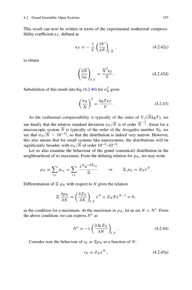
This result can now be written in terms of the experimental isothermal compressibility coefficient κ T , defined as
κ T ≡ −
1
V
∂V
∂P
T ,N
,
(4.2.42c)
to obtain
∂N
∂μ
T ,V
=
N
2 κ T
V
.
(4.2.42d)
Substitution of this result into Eq. (4.2.40) for σ 2
N gives
σ N
N
2
=
k B T κ T
V
.
(4.2.43)
As the isothermal compressibility is typically of the order of V /(Nk B T ), we
see finally that the relative standard deviation σ N /N is of order N
−
1
2 . Since for a
macroscopic system N is typically of the order of the Avogadro number N 0 , we
see that σ N /N ∼ 10 −12 , so that the distribution is indeed very narrow. However,
this also means that for small systems like nanosystems, the distributions will be
significantly broader, with σ N /N of order 10 −4 –10 −6 .
Let us also examine the behaviour of the grand (canonical) distribution in the
neighbourhood of its maximum. From the defining relation for p N , we may write
p N ≡
r N
p r N =
r N
λ N e
−βE r N
⇒
p N = Z N λ
N .
Differentiation of p N with respect to N gives the relation
∂p N
∂N
=
∂Z N
∂N
T ,V
λ
N
+ Z N Nλ
N −1
= 0 ,
as the condition for a maximum. At the maximum in p N , let us set N = N ∗ . From
the above condition, we can express N ∗ as
N
∗
= −λ
∂ ln Z N
∂N
T ,V
.
(4.2.44)
Consider now the behaviour of t N ≡ p N as a function of N:
t N = Z N λ
N ,
(4.2.45a)
197
This result can now be written in terms of the experimental isothermal compressibility coefficient κ T , defined as
κ T ≡ −
1
V
∂V
∂P
T ,N
,
(4.2.42c)
to obtain
∂N
∂μ
T ,V
=
N
2 κ T
V
.
(4.2.42d)
Substitution of this result into Eq. (4.2.40) for σ 2
N gives
σ N
N
2
=
k B T κ T
V
.
(4.2.43)
As the isothermal compressibility is typically of the order of V /(Nk B T ), we
see finally that the relative standard deviation σ N /N is of order N
−
1
2 . Since for a
macroscopic system N is typically of the order of the Avogadro number N 0 , we
see that σ N /N ∼ 10 −12 , so that the distribution is indeed very narrow. However,
this also means that for small systems like nanosystems, the distributions will be
significantly broader, with σ N /N of order 10 −4 –10 −6 .
Let us also examine the behaviour of the grand (canonical) distribution in the
neighbourhood of its maximum. From the defining relation for p N , we may write
p N ≡
r N
p r N =
r N
λ N e
−βE r N
⇒
p N = Z N λ
N .
Differentiation of p N with respect to N gives the relation
∂p N
∂N
=
∂Z N
∂N
T ,V
λ
N
+ Z N Nλ
N −1
= 0 ,
as the condition for a maximum. At the maximum in p N , let us set N = N ∗ . From
the above condition, we can express N ∗ as
N
∗
= −λ
∂ ln Z N
∂N
T ,V
.
(4.2.44)
Consider now the behaviour of t N ≡ p N as a function of N:
t N = Z N λ
N ,
(4.2.45a)