

158
3 Ensembles: Systems of Particles
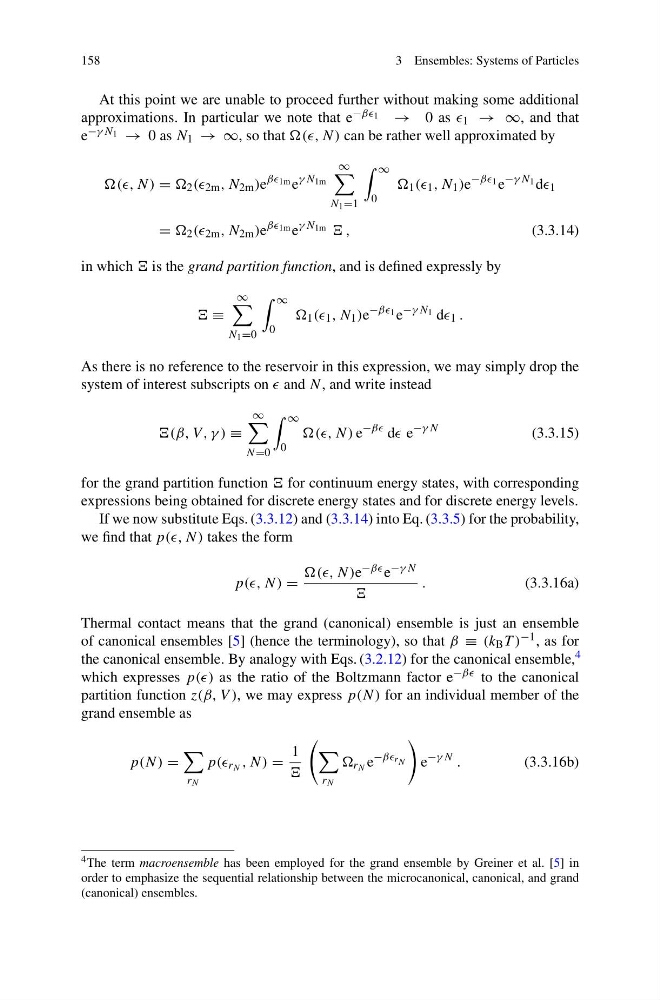
At this point we are unable to proceed further without making some additional
approximations. In particular we note that e −ββ 1 → 0 as 1 → ∞, and that
e −γ N 1 → 0 as N 1 → ∞, so that ((, N) can be rather well approximated by
((, N) = 2 (( 2m , N 2m )e
ββ 1m e
γ N 1m
∞
N 1 =1
∞
0
1 (( 1 , N 1 )e
−ββ 1 e
−γ N 1 d 1
= 2 (( 2m , N 2m )e
ββ 1m e
γ N 1m ,
(3.3.14)
in which is the grand partition function, and is defined expressly by
≡
∞
N 1 =0
∞
0
1 (( 1 , N 1 )e
−ββ 1 e
−γ N 1 d 1 .
As there is no reference to the reservoir in this expression, we may simply drop the
system of interest subscripts on and N , and write instead
V , γ ) ≡
∞
N =0
∞
0
((, N) e
−ββ d e
−γ N
(3.3.15)
for the grand partition function for continuum energy states, with corresponding
expressions being obtained for discrete energy states and for discrete energy levels.
If we now substitute Eqs. (3.3.12) and (3.3.14) into Eq. (3.3.5) for the probability,
we find that p((, N) takes the form
p((, N) =
(, N)e −ββ e −γ N
.
(3.3.16a)
Thermal contact means that the grand (canonical) ensemble is just an ensemble
of canonical ensembles [5] (hence the terminology), so that β ≡ (k B T ) −1 , as for
the canonical ensemble. By analogy with Eqs. (3.2.12) for the canonical ensemble, 4
which expresses p(() as the ratio of the Boltzmann factor e −ββ to the canonical
partition function z(β, V ), we may express p(N) for an individual member of the
grand ensemble as
p(N) =
r N
p(( r N , N) =
1
r N
r N e
−ββ r N
e
−γ N .
(3.3.16b)
4 The term macroensemble has been employed for the grand ensemble by Greiner et al. [5] in
order to emphasize the sequential relationship between the microcanonical, canonical, and grand
(canonical) ensembles.
3 Ensembles: Systems of Particles
At this point we are unable to proceed further without making some additional
approximations. In particular we note that e −ββ 1 → 0 as 1 → ∞, and that
e −γ N 1 → 0 as N 1 → ∞, so that ((, N) can be rather well approximated by
((, N) = 2 (( 2m , N 2m )e
ββ 1m e
γ N 1m
∞
N 1 =1
∞
0
1 (( 1 , N 1 )e
−ββ 1 e
−γ N 1 d 1
= 2 (( 2m , N 2m )e
ββ 1m e
γ N 1m ,
(3.3.14)
in which is the grand partition function, and is defined expressly by
≡
∞
N 1 =0
∞
0
1 (( 1 , N 1 )e
−ββ 1 e
−γ N 1 d 1 .
As there is no reference to the reservoir in this expression, we may simply drop the
system of interest subscripts on and N , and write instead
V , γ ) ≡
∞
N =0
∞
0
((, N) e
−ββ d e
−γ N
(3.3.15)
for the grand partition function for continuum energy states, with corresponding
expressions being obtained for discrete energy states and for discrete energy levels.
If we now substitute Eqs. (3.3.12) and (3.3.14) into Eq. (3.3.5) for the probability,
we find that p((, N) takes the form
p((, N) =
(, N)e −ββ e −γ N
.
(3.3.16a)
Thermal contact means that the grand (canonical) ensemble is just an ensemble
of canonical ensembles [5] (hence the terminology), so that β ≡ (k B T ) −1 , as for
the canonical ensemble. By analogy with Eqs. (3.2.12) for the canonical ensemble, 4
which expresses p(() as the ratio of the Boltzmann factor e −ββ to the canonical
partition function z(β, V ), we may express p(N) for an individual member of the
grand ensemble as
p(N) =
r N
p(( r N , N) =
1
r N
r N e
−ββ r N
e
−γ N .
(3.3.16b)
4 The term macroensemble has been employed for the grand ensemble by Greiner et al. [5] in
order to emphasize the sequential relationship between the microcanonical, canonical, and grand
(canonical) ensembles.