

3.1 Scattering Amplitudes on Moduli Space
77
The amplitude can be rewritten in two different ways. First, the ghost insertions
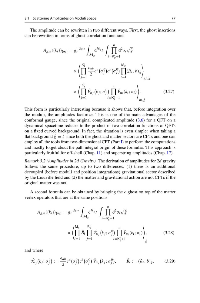
can be rewritten in terms of ghost correlation functions
A g,n ({k i }) {α i } = g
−χ g,n
s
M g
d
M g t
n
i=K c
g +1
d
2 σ i
ˆ
g
×
K c
g
j =1
ab
2
c
a
σ
0
j
c
b
σ
0
j
M g
i=1
( ˆ
μ i , b) ˆ
g
gh, ˆ
g
×
K c
g
j =1
ˆ
V α j
k j ; σ
0
j
n
i=K c
g +1
ˆ
V α i (k i ; σ i )
m, ˆ
g
.
(3.27)
This form is particularly interesting because it shows that, before integration over
the moduli, the amplitudes factorize. This is one of the main advantages of the
conformal gauge, since the original complicated amplitude (3.6) for a QFT on a
dynamical spacetime reduces to the product of two correlation functions of QFTs
on a fixed curved background. In fact, the situation is even simpler when taking a
flat background ˆ
g = δ since both the ghost and matter sectors are CFTs and one can
employ all the tools from two-dimensional CFT (Part I) to perform the computations
and mostly forget about the path integral origin of these formulas. This approach is
particularly fruitful for off-shell (Chap. 11) and superstring amplitudes (Chap. 17).
Remark 3.2 (Amplitudes in 2d Gravity) The derivation of amplitudes for 2d gravity
follows the same procedure, up to two differences: (1) there is an additional
decoupled (before moduli and position integrations) gravitational sector described
by the Liouville field and (2) the matter and gravitational action are not CFTs if the
original matter was not.
A second formula can be obtained by bringing the c ghost on top of the matter
vertex operators that are at the same positions
A g,n ({k i }) {α i } = g
−χ g,n
s
M g
d
M g t
n
i=K c
g +1
d
2 σ i
ˆ
g
×
M g
i=1
ˆ
B i
K c
g
j =1
ˆ
V α j
k j ; σ
0
j
n
i=K c
g +1
ˆ
V α i (k i ; σ i )
ˆ
g
,
(3.28)
and where
ˆ
V α j
k j ; σ
0
j
:=
ab
2
c
a
σ
0
j
c
b
σ
0
j
ˆ
V α j
k j ; σ
0
j
,
ˆ
B i := ( ˆ
μ i , b) ˆ
g .
(3.29)
77
The amplitude can be rewritten in two different ways. First, the ghost insertions
can be rewritten in terms of ghost correlation functions
A g,n ({k i }) {α i } = g
−χ g,n
s
M g
d
M g t
n
i=K c
g +1
d
2 σ i
ˆ
g
×
K c
g
j =1
ab
2
c
a
σ
0
j
c
b
σ
0
j
M g
i=1
( ˆ
μ i , b) ˆ
g
gh, ˆ
g
×
K c
g
j =1
ˆ
V α j
k j ; σ
0
j
n
i=K c
g +1
ˆ
V α i (k i ; σ i )
m, ˆ
g
.
(3.27)
This form is particularly interesting because it shows that, before integration over
the moduli, the amplitudes factorize. This is one of the main advantages of the
conformal gauge, since the original complicated amplitude (3.6) for a QFT on a
dynamical spacetime reduces to the product of two correlation functions of QFTs
on a fixed curved background. In fact, the situation is even simpler when taking a
flat background ˆ
g = δ since both the ghost and matter sectors are CFTs and one can
employ all the tools from two-dimensional CFT (Part I) to perform the computations
and mostly forget about the path integral origin of these formulas. This approach is
particularly fruitful for off-shell (Chap. 11) and superstring amplitudes (Chap. 17).
Remark 3.2 (Amplitudes in 2d Gravity) The derivation of amplitudes for 2d gravity
follows the same procedure, up to two differences: (1) there is an additional
decoupled (before moduli and position integrations) gravitational sector described
by the Liouville field and (2) the matter and gravitational action are not CFTs if the
original matter was not.
A second formula can be obtained by bringing the c ghost on top of the matter
vertex operators that are at the same positions
A g,n ({k i }) {α i } = g
−χ g,n
s
M g
d
M g t
n
i=K c
g +1
d
2 σ i
ˆ
g
×
M g
i=1
ˆ
B i
K c
g
j =1
ˆ
V α j
k j ; σ
0
j
n
i=K c
g +1
ˆ
V α i (k i ; σ i )
ˆ
g
,
(3.28)
and where
ˆ
V α j
k j ; σ
0
j
:=
ab
2
c
a
σ
0
j
c
b
σ
0
j
ˆ
V α j
k j ; σ
0
j
,
ˆ
B i := ( ˆ
μ i , b) ˆ
g .
(3.29)