

C Quantum Field Theory
397
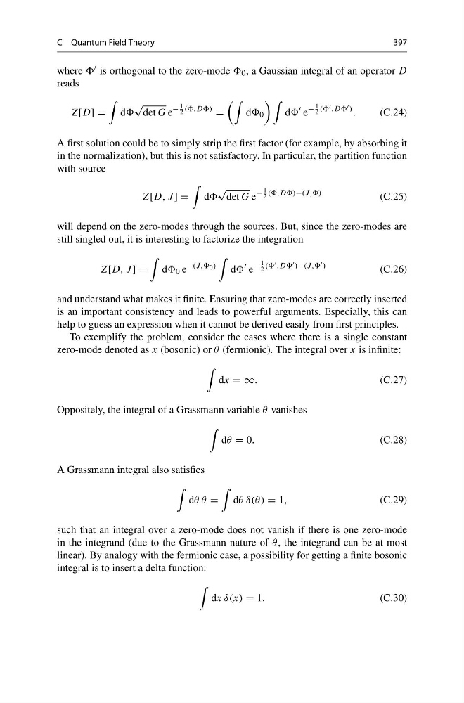
where is orthogonal to the zero-mode 0 , a Gaussian integral of an operator D
reads
Z[D] =
d
√
det G e
−
1
2 ((,DD)
=
d 0
d
e
−
1
2 (( ,DD ) .
(C.24)
A first solution could be to simply strip the first factor (for example, by absorbing it
in the normalization), but this is not satisfactory. In particular, the partition function
with source
Z[D, J ] =
d
√
det G e
−
1
2 ((,DD)−(J,,)
(C.25)
will depend on the zero-modes through the sources. But, since the zero-modes are
still singled out, it is interesting to factorize the integration
Z[D, J ] =
d 0 e
−(J,, 0 )
d
e
−
1
2 (( ,DD )−(J,, )
(C.26)
and understand what makes it finite. Ensuring that zero-modes are correctly inserted
is an important consistency and leads to powerful arguments. Especially, this can
help to guess an expression when it cannot be derived easily from first principles.
To exemplify the problem, consider the cases where there is a single constant
zero-mode denoted as x (bosonic) or θ (fermionic). The integral over x is infinite:
dx = ∞.
(C.27)
Oppositely, the integral of a Grassmann variable θ vanishes
dθ = 0.
(C.28)
A Grassmann integral also satisfies
dθ θ =
dθ δ(θ) = 1,
(C.29)
such that an integral over a zero-mode does not vanish if there is one zero-mode
in the integrand (due to the Grassmann nature of θ , the integrand can be at most
linear). By analogy with the fermionic case, a possibility for getting a finite bosonic
integral is to insert a delta function:
dx δ(x) = 1.
(C.30)
397
where is orthogonal to the zero-mode 0 , a Gaussian integral of an operator D
reads
Z[D] =
d
√
det G e
−
1
2 ((,DD)
=
d 0
d
e
−
1
2 (( ,DD ) .
(C.24)
A first solution could be to simply strip the first factor (for example, by absorbing it
in the normalization), but this is not satisfactory. In particular, the partition function
with source
Z[D, J ] =
d
√
det G e
−
1
2 ((,DD)−(J,,)
(C.25)
will depend on the zero-modes through the sources. But, since the zero-modes are
still singled out, it is interesting to factorize the integration
Z[D, J ] =
d 0 e
−(J,, 0 )
d
e
−
1
2 (( ,DD )−(J,, )
(C.26)
and understand what makes it finite. Ensuring that zero-modes are correctly inserted
is an important consistency and leads to powerful arguments. Especially, this can
help to guess an expression when it cannot be derived easily from first principles.
To exemplify the problem, consider the cases where there is a single constant
zero-mode denoted as x (bosonic) or θ (fermionic). The integral over x is infinite:
dx = ∞.
(C.27)
Oppositely, the integral of a Grassmann variable θ vanishes
dθ = 0.
(C.28)
A Grassmann integral also satisfies
dθ θ =
dθ δ(θ) = 1,
(C.29)
such that an integral over a zero-mode does not vanish if there is one zero-mode
in the integrand (due to the Grassmann nature of θ , the integrand can be at most
linear). By analogy with the fermionic case, a possibility for getting a finite bosonic
integral is to insert a delta function:
dx δ(x) = 1.
(C.30)