

294
14 Amplitude Factorization and Feynman Diagrams
Feynman graphs. Then, the goal is to find the Feynman rules of the theory: since the
propagator has already been identified (further studied in Sect. 14.2.2), it is sufficient
to find the interaction vertices.
Let us make this more precise by considering an amplitude A g,n (V 1 , . . . , V n ).
The index of an amplitude is defined to be the index (12.50) of the corresponding
Riemann surfaces
r(A g,n ) := r(( g,n ) = 3g + n − 2.
(14.32)
Contributions to an amplitude with a given r(A g,n ) can be described in terms of
amplitudes A g ,n with r(A g ,n ) < r(A g,n ). But, the moduli space M g,n cannot
(generically) be completely covered with the plumbing fixture of lower-dimensional
moduli spaces, i.e. with r(M g ,n ) < r(M g,n ) (Sect. 12.3.3). Then, the same must
be true for the amplitudes, such that A g,n cannot be uniquely expressed in terms of
amplitudes A g ,n .
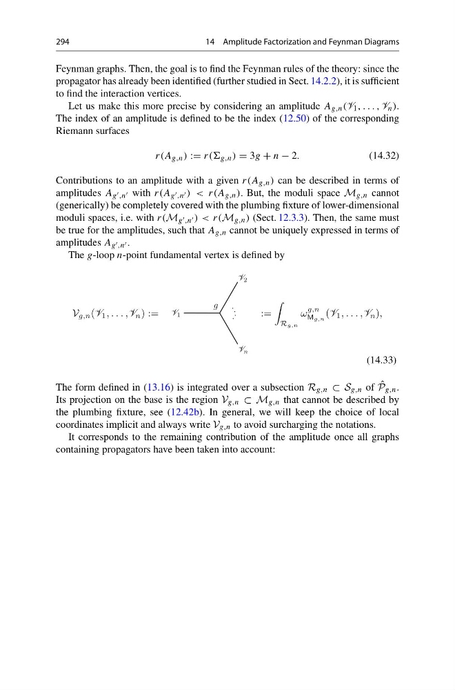
The g-loop n-point fundamental vertex is defined by
V g,n
) :=
:=
Rg,n
ω
g,n
Mg,n
),
( , . . . , n
1
( , . . . , n
1
(14.33)
The form defined in (13.16) is integrated over a subsection R g,n ⊂ S g,n of ˆ
P g,n .
Its projection on the base is the region V g,n ⊂ M g,n that cannot be described by
the plumbing fixture, see (12.42b). In general, we will keep the choice of local
coordinates implicit and always write V g,n to avoid surcharging the notations.
It corresponds to the remaining contribution of the amplitude once all graphs
containing propagators have been taken into account:
14 Amplitude Factorization and Feynman Diagrams
Feynman graphs. Then, the goal is to find the Feynman rules of the theory: since the
propagator has already been identified (further studied in Sect. 14.2.2), it is sufficient
to find the interaction vertices.
Let us make this more precise by considering an amplitude A g,n (V 1 , . . . , V n ).
The index of an amplitude is defined to be the index (12.50) of the corresponding
Riemann surfaces
r(A g,n ) := r(( g,n ) = 3g + n − 2.
(14.32)
Contributions to an amplitude with a given r(A g,n ) can be described in terms of
amplitudes A g ,n with r(A g ,n ) < r(A g,n ). But, the moduli space M g,n cannot
(generically) be completely covered with the plumbing fixture of lower-dimensional
moduli spaces, i.e. with r(M g ,n ) < r(M g,n ) (Sect. 12.3.3). Then, the same must
be true for the amplitudes, such that A g,n cannot be uniquely expressed in terms of
amplitudes A g ,n .
The g-loop n-point fundamental vertex is defined by
V g,n
) :=
:=
Rg,n
ω
g,n
Mg,n
),
( , . . . , n
1
( , . . . , n
1
(14.33)
The form defined in (13.16) is integrated over a subsection R g,n ⊂ S g,n of ˆ
P g,n .
Its projection on the base is the region V g,n ⊂ M g,n that cannot be described by
the plumbing fixture, see (12.42b). In general, we will keep the choice of local
coordinates implicit and always write V g,n to avoid surcharging the notations.
It corresponds to the remaining contribution of the amplitude once all graphs
containing propagators have been taken into account: