

14.2 Feynman Diagrams and Feynman Rules
295
=
0≤h≤g
0≤m
+ perms +
(14.34)
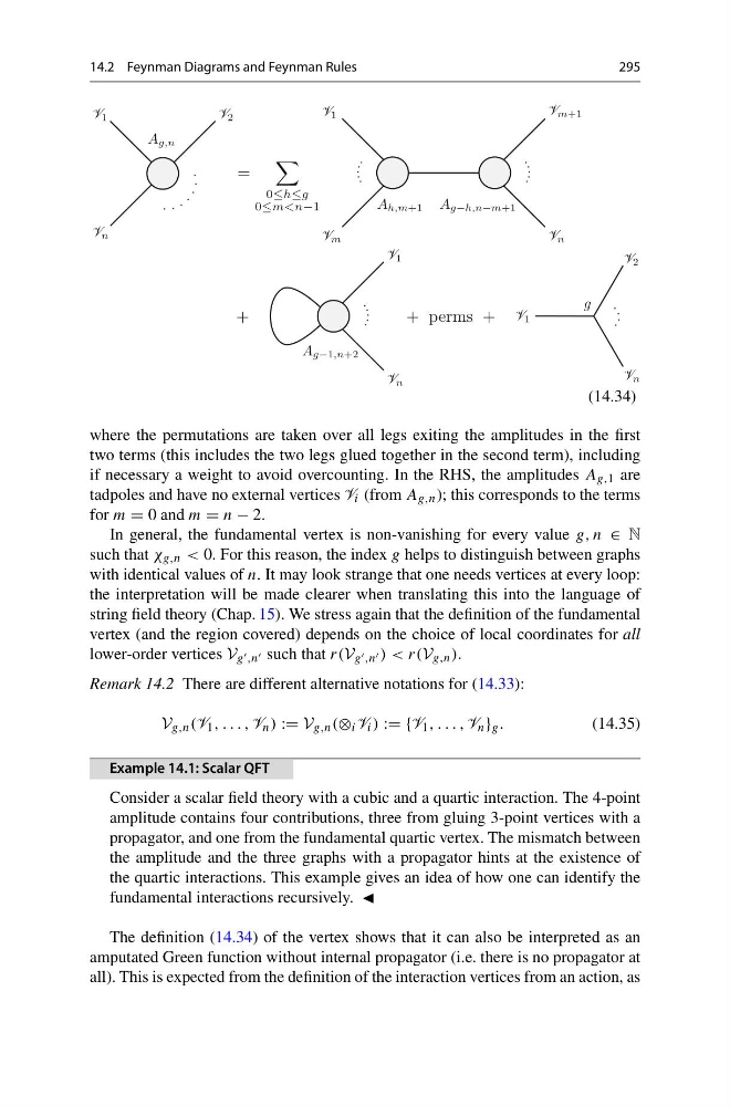
where the permutations are taken over all legs exiting the amplitudes in the first
two terms (this includes the two legs glued together in the second term), including
if necessary a weight to avoid overcounting. In the RHS, the amplitudes A g,1 are
tadpoles and have no external vertices V i (from A g,n ); this corresponds to the terms
for m = 0 and m = n − 2.
In general, the fundamental vertex is non-vanishing for every value g, n ∈ N
such that χ g,n < 0. For this reason, the index g helps to distinguish between graphs
with identical values of n. It may look strange that one needs vertices at every loop:
the interpretation will be made clearer when translating this into the language of
string field theory (Chap. 15). We stress again that the definition of the fundamental
vertex (and the region covered) depends on the choice of local coordinates for all
lower-order vertices V g ,n such that r(V g ,n ) < r(V g,n ).
Remark 14.2 There are different alternative notations for (14.33):
V g,n (V 1 , . . . , V n ) := V g,n (⊗ i V i ) := {V 1 , . . . , V n } g .
(14.35)
Example 14.1: Scalar QFT
Consider a scalar field theory with a cubic and a quartic interaction. The 4-point
amplitude contains four contributions, three from gluing 3-point vertices with a
propagator, and one from the fundamental quartic vertex. The mismatch between
the amplitude and the three graphs with a propagator hints at the existence of
the quartic interactions. This example gives an idea of how one can identify the
fundamental interactions recursively.
The definition (14.34) of the vertex shows that it can also be interpreted as an
amputated Green function without internal propagator (i.e. there is no propagator at
all). This is expected from the definition of the interaction vertices from an action, as
295
=
0≤h≤g
0≤m
+ perms +
(14.34)
where the permutations are taken over all legs exiting the amplitudes in the first
two terms (this includes the two legs glued together in the second term), including
if necessary a weight to avoid overcounting. In the RHS, the amplitudes A g,1 are
tadpoles and have no external vertices V i (from A g,n ); this corresponds to the terms
for m = 0 and m = n − 2.
In general, the fundamental vertex is non-vanishing for every value g, n ∈ N
such that χ g,n < 0. For this reason, the index g helps to distinguish between graphs
with identical values of n. It may look strange that one needs vertices at every loop:
the interpretation will be made clearer when translating this into the language of
string field theory (Chap. 15). We stress again that the definition of the fundamental
vertex (and the region covered) depends on the choice of local coordinates for all
lower-order vertices V g ,n such that r(V g ,n ) < r(V g,n ).
Remark 14.2 There are different alternative notations for (14.33):
V g,n (V 1 , . . . , V n ) := V g,n (⊗ i V i ) := {V 1 , . . . , V n } g .
(14.35)
Example 14.1: Scalar QFT
Consider a scalar field theory with a cubic and a quartic interaction. The 4-point
amplitude contains four contributions, three from gluing 3-point vertices with a
propagator, and one from the fundamental quartic vertex. The mismatch between
the amplitude and the three graphs with a propagator hints at the existence of
the quartic interactions. This example gives an idea of how one can identify the
fundamental interactions recursively.
The definition (14.34) of the vertex shows that it can also be interpreted as an
amputated Green function without internal propagator (i.e. there is no propagator at
all). This is expected from the definition of the interaction vertices from an action, as