

14.2 Feynman Diagrams and Feynman Rules
293
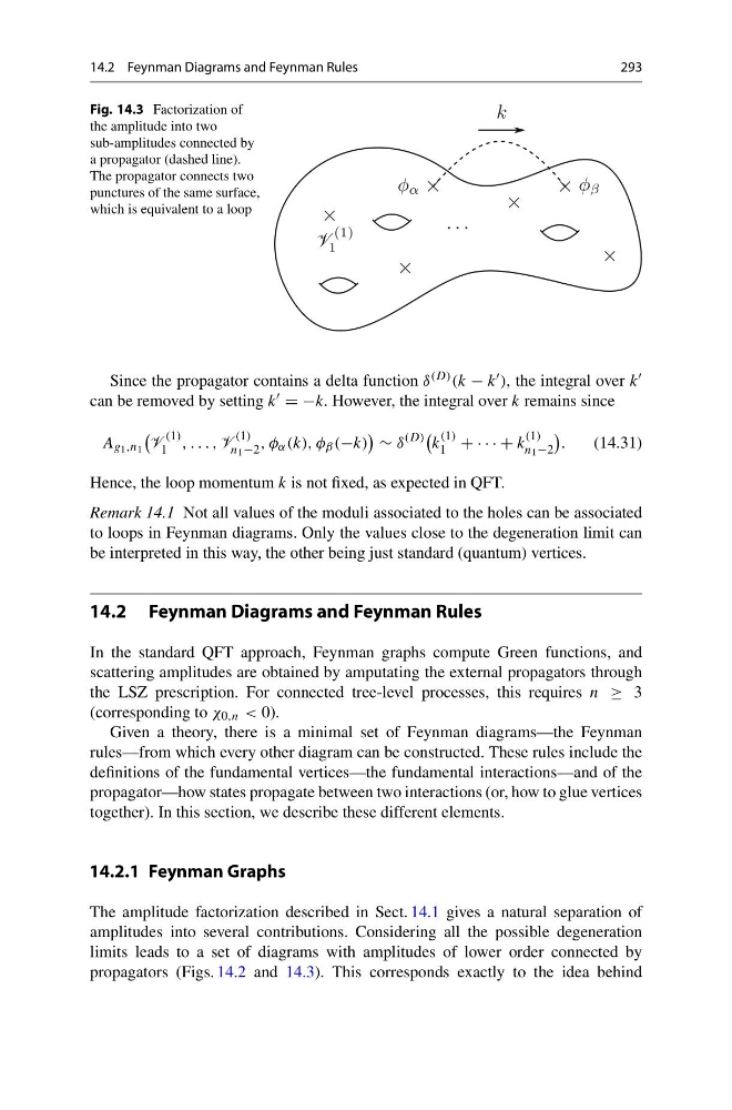
Fig. 14.3 Factorization of
the amplitude into two
sub-amplitudes connected by
a propagator (dashed line).
The propagator connects two
punctures of the same surface,
which is equivalent to a loop
Since the propagator contains a delta function δ (D) (k − k ), the integral over k
can be removed by setting k = −k. However, the integral over k remains since
A g 1 ,n 1
V
(1)
1 , . . . , V
(1)
n 1 −2 , φ α (k), φ β (−k)
∼ δ
(D)
k
(1)
1 + · · · + k
(1)
n 1 −2
.
(14.31)
Hence, the loop momentum k is not fixed, as expected in QFT.
Remark 14.1 Not all values of the moduli associated to the holes can be associated
to loops in Feynman diagrams. Only the values close to the degeneration limit can
be interpreted in this way, the other being just standard (quantum) vertices.
14.2 Feynman Diagrams and Feynman Rules
In the standard QFT approach, Feynman graphs compute Green functions, and
scattering amplitudes are obtained by amputating the external propagators through
the LSZ prescription. For connected tree-level processes, this requires n ≥ 3
(corresponding to χ 0,n < 0).
Given a theory, there is a minimal set of Feynman diagrams—the Feynman
rules—from which every other diagram can be constructed. These rules include the
definitions of the fundamental vertices—the fundamental interactions—and of the
propagator—how states propagate between two interactions (or, how to glue vertices
together). In this section, we describe these different elements.
14.2.1 Feynman Graphs
The amplitude factorization described in Sect. 14.1 gives a natural separation of
amplitudes into several contributions. Considering all the possible degeneration
limits leads to a set of diagrams with amplitudes of lower order connected by
propagators (Figs. 14.2 and 14.3). This corresponds exactly to the idea behind
293
Fig. 14.3 Factorization of
the amplitude into two
sub-amplitudes connected by
a propagator (dashed line).
The propagator connects two
punctures of the same surface,
which is equivalent to a loop
Since the propagator contains a delta function δ (D) (k − k ), the integral over k
can be removed by setting k = −k. However, the integral over k remains since
A g 1 ,n 1
V
(1)
1 , . . . , V
(1)
n 1 −2 , φ α (k), φ β (−k)
∼ δ
(D)
k
(1)
1 + · · · + k
(1)
n 1 −2
.
(14.31)
Hence, the loop momentum k is not fixed, as expected in QFT.
Remark 14.1 Not all values of the moduli associated to the holes can be associated
to loops in Feynman diagrams. Only the values close to the degeneration limit can
be interpreted in this way, the other being just standard (quantum) vertices.
14.2 Feynman Diagrams and Feynman Rules
In the standard QFT approach, Feynman graphs compute Green functions, and
scattering amplitudes are obtained by amputating the external propagators through
the LSZ prescription. For connected tree-level processes, this requires n ≥ 3
(corresponding to χ 0,n < 0).
Given a theory, there is a minimal set of Feynman diagrams—the Feynman
rules—from which every other diagram can be constructed. These rules include the
definitions of the fundamental vertices—the fundamental interactions—and of the
propagator—how states propagate between two interactions (or, how to glue vertices
together). In this section, we describe these different elements.
14.2.1 Feynman Graphs
The amplitude factorization described in Sect. 14.1 gives a natural separation of
amplitudes into several contributions. Considering all the possible degeneration
limits leads to a set of diagrams with amplitudes of lower order connected by
propagators (Figs. 14.2 and 14.3). This corresponds exactly to the idea behind