

14.1 Amplitude Factorization
289
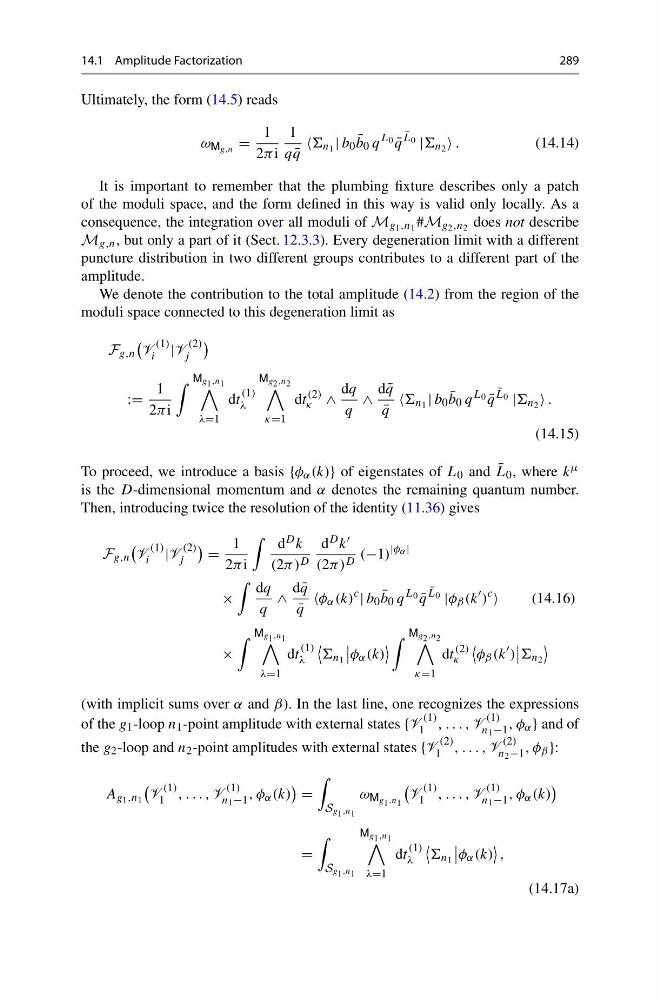
Ultimately, the form (14.5) reads
ω M g,n =
1
2π i
1
q ¯
q
n 1 | b 0 ¯
b 0 q
L 0 ¯
q
¯
L 0 | n 2 .
(14.14)
It is important to remember that the plumbing fixture describes only a patch
of the moduli space, and the form defined in this way is valid only locally. As a
consequence, the integration over all moduli of M g 1 ,n 1 #M g 2 ,n 2 does not describe
M g,n , but only a part of it (Sect. 12.3.3). Every degeneration limit with a different
puncture distribution in two different groups contributes to a different part of the
amplitude.
We denote the contribution to the total amplitude (14.2) from the region of the
moduli space connected to this degeneration limit as
F g,n
V
(1)
i |V
(2)
j
:=
1
2π i
M g 1 ,n 1
λ=1
dt
(1)
λ
M g 2 ,n 2
κ=1
dt
(2)
κ ∧
dq
q
∧
d ¯
q
¯
q
n 1 | b 0 ¯
b 0 q
L 0 ¯
q
¯
L 0 | n 2 .
(14.15)
To proceed, we introduce a basis {φ α (k)} of eigenstates of L 0 and ¯
L 0 , where k μ
is the D-dimensional momentum and α denotes the remaining quantum number.
Then, introducing twice the resolution of the identity (11.36) gives
F g,n
V
(1)
i |V
(2)
j
=
1
2π i
d D k
(2π) D
d D k
(2π) D (−1)
|φ α |
×
dq
q
∧
d ¯
q
¯
q
φ α (k)
c
| b 0 ¯
b 0 q
L 0 ¯
q
¯
L 0 |φ β (k
)
c
(14.16)
×
M g 1 ,n 1
λ=1
dt
(1)
λ
n 1
φ α (k)
M g 2 ,n 2
κ=1
dt
(2)
κ
φ β (k
)
n 2
(with implicit sums over α and β). In the last line, one recognizes the expressions
of the g 1 -loop n 1 -point amplitude with external states {V
(1)
1 , . . . , V
(1)
n 1 −1 , φ α } and of
the g 2 -loop and n 2 -point amplitudes with external states {V
(2)
1 , . . . , V
(2)
n 2 −1 , φ β }:
A g 1 ,n 1
V
(1)
1 , . . . , V
(1)
n 1 −1 , φ α (k)
=
S g 1 ,n 1
ω M g 1 ,n 1
V
(1)
1 , . . . , V
(1)
n 1 −1 , φ α (k)
=
S g 1 ,n 1
M g 1 ,n 1
λ=1
dt
(1)
λ
n 1
φ α (k)
,
(14.17a)
289
Ultimately, the form (14.5) reads
ω M g,n =
1
2π i
1
q ¯
q
n 1 | b 0 ¯
b 0 q
L 0 ¯
q
¯
L 0 | n 2 .
(14.14)
It is important to remember that the plumbing fixture describes only a patch
of the moduli space, and the form defined in this way is valid only locally. As a
consequence, the integration over all moduli of M g 1 ,n 1 #M g 2 ,n 2 does not describe
M g,n , but only a part of it (Sect. 12.3.3). Every degeneration limit with a different
puncture distribution in two different groups contributes to a different part of the
amplitude.
We denote the contribution to the total amplitude (14.2) from the region of the
moduli space connected to this degeneration limit as
F g,n
V
(1)
i |V
(2)
j
:=
1
2π i
M g 1 ,n 1
λ=1
dt
(1)
λ
M g 2 ,n 2
κ=1
dt
(2)
κ ∧
dq
q
∧
d ¯
q
¯
q
n 1 | b 0 ¯
b 0 q
L 0 ¯
q
¯
L 0 | n 2 .
(14.15)
To proceed, we introduce a basis {φ α (k)} of eigenstates of L 0 and ¯
L 0 , where k μ
is the D-dimensional momentum and α denotes the remaining quantum number.
Then, introducing twice the resolution of the identity (11.36) gives
F g,n
V
(1)
i |V
(2)
j
=
1
2π i
d D k
(2π) D
d D k
(2π) D (−1)
|φ α |
×
dq
q
∧
d ¯
q
¯
q
φ α (k)
c
| b 0 ¯
b 0 q
L 0 ¯
q
¯
L 0 |φ β (k
)
c
(14.16)
×
M g 1 ,n 1
λ=1
dt
(1)
λ
n 1
φ α (k)
M g 2 ,n 2
κ=1
dt
(2)
κ
φ β (k
)
n 2
(with implicit sums over α and β). In the last line, one recognizes the expressions
of the g 1 -loop n 1 -point amplitude with external states {V
(1)
1 , . . . , V
(1)
n 1 −1 , φ α } and of
the g 2 -loop and n 2 -point amplitudes with external states {V
(2)
1 , . . . , V
(2)
n 2 −1 , φ β }:
A g 1 ,n 1
V
(1)
1 , . . . , V
(1)
n 1 −1 , φ α (k)
=
S g 1 ,n 1
ω M g 1 ,n 1
V
(1)
1 , . . . , V
(1)
n 1 −1 , φ α (k)
=
S g 1 ,n 1
M g 1 ,n 1
λ=1
dt
(1)
λ
n 1
φ α (k)
,
(14.17a)