

288
14 Amplitude Factorization and Feynman Diagrams
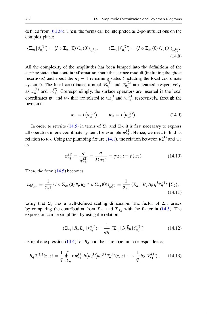
defined from (6.136). Then, the forms can be interpreted as 2-point functions on the
complex plane:
n 1 |V
(1)
n 1
= =I ◦ n 1 (0)V n 1 (0) w
(1)
n 1
,
n 2 |V
(2)
n 2
= =I ◦ n 2 (0)V n 2 (0) w
(2)
n 2
.
(14.8)
All the complexity of the amplitudes has been lumped into the definitions of the
surface states that contain information about the surface moduli (including the ghost
insertions) and about the n 1 − 1 remaining states (including the local coordinate
systems). The local coordinates around V
(1)
n 1 and V
(2)
n 2 are denoted, respectively,
as w
(1)
n 1 and w
(2)
n 2 . Correspondingly, the surface operators are inserted in the local
coordinates w 1 and w 2 that are related to w
(1)
n 1 and w
(2)
n 2 , respectively, through the
inversion:
w 1 = I
w
(1)
n 1
,
w 2 = I
w
(2)
n 2
.
(14.9)
In order to rewrite (14.5) in terms of 1 and 2 , it is first necessary to express
all operators in one coordinate system, for example w
(1)
n 1 . Hence, we need to find its
relation to w 2 . Using the plumbing fixture (14.1), the relation between w
(1)
n 1 and w 2
is:
w
(1)
n 1
=
q
w
(2)
n 2
=
q
I (w 2 )
= qw 2 := f (w 2 ).
(14.10)
Then, the form (14.5) becomes
ω M g,n =
1
2π i
I ◦ n 1 (0)B q B ¯
q f ◦ n 2 (0) w
(1)
n 1
=
1
2π i
n 1 | B q B ¯
q q
L 0 ¯
q
¯
L 0 | 2 ,
(14.11)
using that 2 has a well-defined scaling dimension. The factor of 2π i arises
by comparing the contribution from n 1 and n 2 with the factor in (14.5). The
expression can be simplified by using the relation
n 1 | B q B ¯
q |V
(1)
n 1
=
1
q ¯
q
n 1 | b 0 ¯
b 0 |V
(1)
n 1
(14.12)
using the expression (14.4) for B q and the state–operator correspondence:
B q V
(1)
n 1
(z, ¯
z) =
1
q
C q
dw
(1)
n 1
b
w
(1)
n 1
w
(1)
n 1
V
(1)
n 1
(z, ¯
z) −→
1
q
b 0 |V
(1)
n 1
.
(14.13)
14 Amplitude Factorization and Feynman Diagrams
defined from (6.136). Then, the forms can be interpreted as 2-point functions on the
complex plane:
n 1 |V
(1)
n 1
= =I ◦ n 1 (0)V n 1 (0) w
(1)
n 1
,
n 2 |V
(2)
n 2
= =I ◦ n 2 (0)V n 2 (0) w
(2)
n 2
.
(14.8)
All the complexity of the amplitudes has been lumped into the definitions of the
surface states that contain information about the surface moduli (including the ghost
insertions) and about the n 1 − 1 remaining states (including the local coordinate
systems). The local coordinates around V
(1)
n 1 and V
(2)
n 2 are denoted, respectively,
as w
(1)
n 1 and w
(2)
n 2 . Correspondingly, the surface operators are inserted in the local
coordinates w 1 and w 2 that are related to w
(1)
n 1 and w
(2)
n 2 , respectively, through the
inversion:
w 1 = I
w
(1)
n 1
,
w 2 = I
w
(2)
n 2
.
(14.9)
In order to rewrite (14.5) in terms of 1 and 2 , it is first necessary to express
all operators in one coordinate system, for example w
(1)
n 1 . Hence, we need to find its
relation to w 2 . Using the plumbing fixture (14.1), the relation between w
(1)
n 1 and w 2
is:
w
(1)
n 1
=
q
w
(2)
n 2
=
q
I (w 2 )
= qw 2 := f (w 2 ).
(14.10)
Then, the form (14.5) becomes
ω M g,n =
1
2π i
I ◦ n 1 (0)B q B ¯
q f ◦ n 2 (0) w
(1)
n 1
=
1
2π i
n 1 | B q B ¯
q q
L 0 ¯
q
¯
L 0 | 2 ,
(14.11)
using that 2 has a well-defined scaling dimension. The factor of 2π i arises
by comparing the contribution from n 1 and n 2 with the factor in (14.5). The
expression can be simplified by using the relation
n 1 | B q B ¯
q |V
(1)
n 1
=
1
q ¯
q
n 1 | b 0 ¯
b 0 |V
(1)
n 1
(14.12)
using the expression (14.4) for B q and the state–operator correspondence:
B q V
(1)
n 1
(z, ¯
z) =
1
q
C q
dw
(1)
n 1
b
w
(1)
n 1
w
(1)
n 1
V
(1)
n 1
(z, ¯
z) −→
1
q
b 0 |V
(1)
n 1
.
(14.13)