

290
14 Amplitude Factorization and Feynman Diagrams
A g 2 ,n 2
V
(2)
1 , . . . , V
(2)
n 2 −1 , φ β (k
)
=
S g 2 ,n 2
ω M g 2 ,n 2
V
(2)
1 , . . . , V
(2)
n 2 −2 , φ β (k
)
=
S g 2 ,n 2
M g 2 ,n 2
λ=1
dt
(2)
λ
n 2
φ β (k
)
.
(14.17b)
The property (B.27) has been used to reverse the order of the BPZ product for the
second Riemann surface, and this cancels the factor (−1) |φ α | .
Defining the second line of (14.16) as
αβ (k, k
) :=
φ α (k)
c , φ β (k
)
c
:=
1
2π i
dq
q
∧
d ¯
q
¯
q
φ α (k)
c
| b 0 ¯
b 0 q
L 0 ¯
q
¯
L 0 |φ β (k
)
c
,
(14.18)
one has
F g,n
V
(1)
i |V
(2)
j
=
d D k
(2π) D
d D k
(2π) D A g 1 ,n 1
V
(1)
1 , . . . , V
(1)
n 1 −1 , φ α (k)
αβ (k, k
)
× A g 2 ,n 2
V
(2)
1 , . . . , V
(2)
n 2 −1 , φ β (k
)
.
(14.19)
We recover the expressions from Sect. 11.1.2, but for a more general amplitude. We
had found that corresponds to the propagator: its properties are studied further in
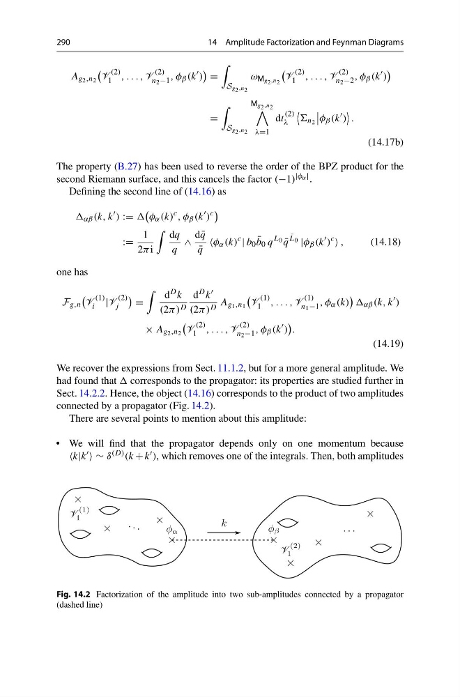
Sect. 14.2.2. Hence, the object (14.16) corresponds to the product of two amplitudes
connected by a propagator (Fig. 14.2).
There are several points to mention about this amplitude:
• We will find that the propagator depends only on one momentum because
k|k ∼ δ (D) (k + k ), which removes one of the integrals. Then, both amplitudes
Fig. 14.2 Factorization of the amplitude into two sub-amplitudes connected by a propagator
(dashed line)
14 Amplitude Factorization and Feynman Diagrams
A g 2 ,n 2
V
(2)
1 , . . . , V
(2)
n 2 −1 , φ β (k
)
=
S g 2 ,n 2
ω M g 2 ,n 2
V
(2)
1 , . . . , V
(2)
n 2 −2 , φ β (k
)
=
S g 2 ,n 2
M g 2 ,n 2
λ=1
dt
(2)
λ
n 2
φ β (k
)
.
(14.17b)
The property (B.27) has been used to reverse the order of the BPZ product for the
second Riemann surface, and this cancels the factor (−1) |φ α | .
Defining the second line of (14.16) as
αβ (k, k
) :=
φ α (k)
c , φ β (k
)
c
:=
1
2π i
dq
q
∧
d ¯
q
¯
q
φ α (k)
c
| b 0 ¯
b 0 q
L 0 ¯
q
¯
L 0 |φ β (k
)
c
,
(14.18)
one has
F g,n
V
(1)
i |V
(2)
j
=
d D k
(2π) D
d D k
(2π) D A g 1 ,n 1
V
(1)
1 , . . . , V
(1)
n 1 −1 , φ α (k)
αβ (k, k
)
× A g 2 ,n 2
V
(2)
1 , . . . , V
(2)
n 2 −1 , φ β (k
)
.
(14.19)
We recover the expressions from Sect. 11.1.2, but for a more general amplitude. We
had found that corresponds to the propagator: its properties are studied further in
Sect. 14.2.2. Hence, the object (14.16) corresponds to the product of two amplitudes
connected by a propagator (Fig. 14.2).
There are several points to mention about this amplitude:
• We will find that the propagator depends only on one momentum because
k|k ∼ δ (D) (k + k ), which removes one of the integrals. Then, both amplitudes
Fig. 14.2 Factorization of the amplitude into two sub-amplitudes connected by a propagator
(dashed line)