

154
7 CFT Systems
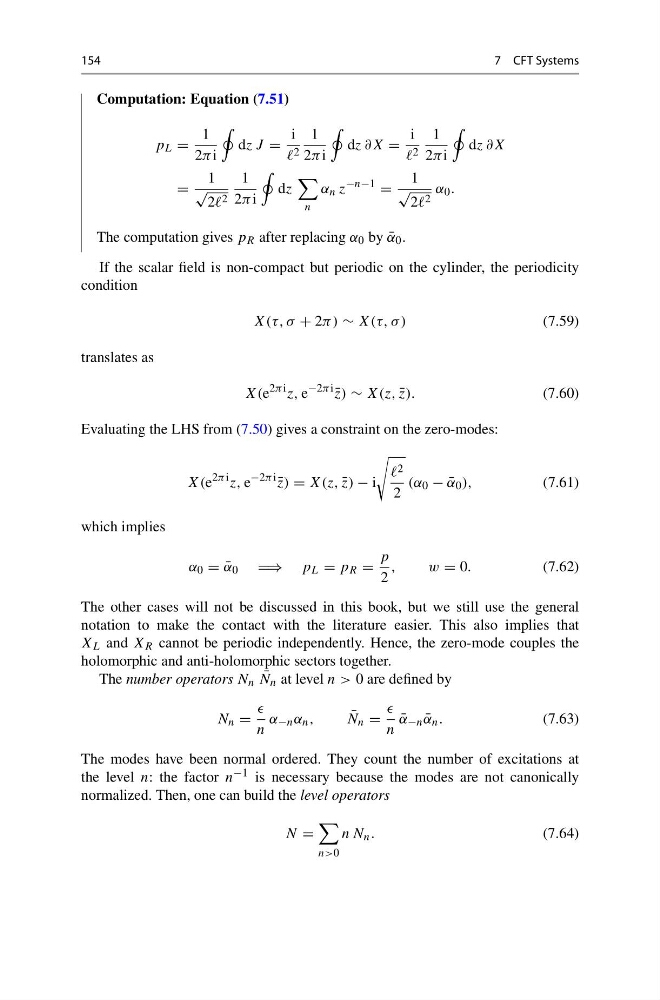
Computation: Equation (7.51)
p L =
1
2π i
dz J =
i
2
1
2π i
dz ∂X =
i
2
1
2π i
dz ∂X
=
1
√
2 2
1
2π i
dz
n
α n z
−n−1
=
1
√
2 2
α 0 .
The computation gives p R after replacing α 0 by ¯
α 0 .
If the scalar field is non-compact but periodic on the cylinder, the periodicity
condition
X(τ, σ + 2π) ∼ X(τ, σ )
(7.59)
translates as
X(e
2π i z, e
−2π i
¯
z) ∼ X(z, ¯
z).
(7.60)
Evaluating the LHS from (7.50) gives a constraint on the zero-modes:
X(e
2π i z, e
−2π i
¯
z) = X(z, ¯
z) − i
2
2
(α 0 − ¯
α 0 ),
(7.61)
which implies
α 0 = ¯
α 0 ⇒ p L = p R =
p
2
,
w= 0.
(7.62)
The other cases will not be discussed in this book, but we still use the general
notation to make the contact with the literature easier. This also implies that
X L and X R cannot be periodic independently. Hence, the zero-mode couples the
holomorphic and anti-holomorphic sectors together.
The number operators N n ¯
N n at level n > 0 are defined by
N n =
n
α −n α n ,
¯
N n =
n
¯
α −n ¯
α n .
(7.63)
The modes have been normal ordered. They count the number of excitations at
the level n: the factor n −1 is necessary because the modes are not canonically
normalized. Then, one can build the level operators
N =
n>0
n N n .
(7.64)
7 CFT Systems
Computation: Equation (7.51)
p L =
1
2π i
dz J =
i
2
1
2π i
dz ∂X =
i
2
1
2π i
dz ∂X
=
1
√
2 2
1
2π i
dz
n
α n z
−n−1
=
1
√
2 2
α 0 .
The computation gives p R after replacing α 0 by ¯
α 0 .
If the scalar field is non-compact but periodic on the cylinder, the periodicity
condition
X(τ, σ + 2π) ∼ X(τ, σ )
(7.59)
translates as
X(e
2π i z, e
−2π i
¯
z) ∼ X(z, ¯
z).
(7.60)
Evaluating the LHS from (7.50) gives a constraint on the zero-modes:
X(e
2π i z, e
−2π i
¯
z) = X(z, ¯
z) − i
2
2
(α 0 − ¯
α 0 ),
(7.61)
which implies
α 0 = ¯
α 0 ⇒ p L = p R =
p
2
,
w= 0.
(7.62)
The other cases will not be discussed in this book, but we still use the general
notation to make the contact with the literature easier. This also implies that
X L and X R cannot be periodic independently. Hence, the zero-mode couples the
holomorphic and anti-holomorphic sectors together.
The number operators N n ¯
N n at level n > 0 are defined by
N n =
n
α −n α n ,
¯
N n =
n
¯
α −n ¯
α n .
(7.63)
The modes have been normal ordered. They count the number of excitations at
the level n: the factor n −1 is necessary because the modes are not canonically
normalized. Then, one can build the level operators
N =
n>0
n N n .
(7.64)