

6. Open the reconstruction software and select the CT image,
send it to batch CT, and reconstruct it to a spatial resolution of
minimum 0.2 mm (see Note 9), using the filtered backprojection (FBP) algorithm.
7. Repeat the steps 3–6 for all the samples (water, solvent, and
each different Me 2 SO concentration).
8. Open the analysis software, and select first the water image.
Select the image scale that allows you to visualize better the
different concentrations (see Note 10). Create a volume of
interest (VOI) with the size and shape according to the
biological sample you are going to analyze and at the same
location where your sample is going to be placed (see Note 11).
Use the statistic tool of the analysis software to get the average
CT values of the VOI and the error, expressed as the standard
deviation of all the CT values of each vowel contained within
the VOI. Write down the average CT values of the sample of
water.
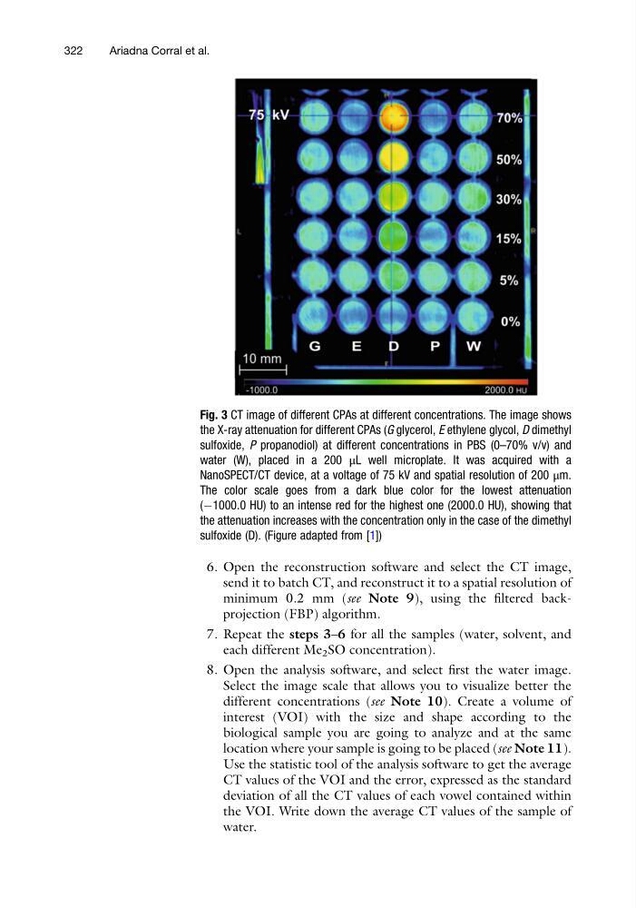
Fig. 3 CT image of different CPAs at different concentrations. The image shows
the X-ray attenuation for different CPAs (G glycerol, E ethylene glycol, D dimethyl
sulfoxide, P propanodiol) at different concentrations in PBS (0–70% v/v) and
water (W), placed in a 200 μL well microplate. It was acquired with a
NanoSPECT/CT device, at a voltage of 75 kV and spatial resolution of 200 μm.
The color scale goes from a dark blue color for the lowest attenuation
(À1000.0 HU) to an intense red for the highest one (2000.0 HU), showing that
the attenuation increases with the concentration only in the case of the dimethyl
sulfoxide (D). (Figure adapted from [1])
322
Ariadna Corral et al.
send it to batch CT, and reconstruct it to a spatial resolution of
minimum 0.2 mm (see Note 9), using the filtered backprojection (FBP) algorithm.
7. Repeat the steps 3–6 for all the samples (water, solvent, and
each different Me 2 SO concentration).
8. Open the analysis software, and select first the water image.
Select the image scale that allows you to visualize better the
different concentrations (see Note 10). Create a volume of
interest (VOI) with the size and shape according to the
biological sample you are going to analyze and at the same
location where your sample is going to be placed (see Note 11).
Use the statistic tool of the analysis software to get the average
CT values of the VOI and the error, expressed as the standard
deviation of all the CT values of each vowel contained within
the VOI. Write down the average CT values of the sample of
water.
Fig. 3 CT image of different CPAs at different concentrations. The image shows
the X-ray attenuation for different CPAs (G glycerol, E ethylene glycol, D dimethyl
sulfoxide, P propanodiol) at different concentrations in PBS (0–70% v/v) and
water (W), placed in a 200 μL well microplate. It was acquired with a
NanoSPECT/CT device, at a voltage of 75 kV and spatial resolution of 200 μm.
The color scale goes from a dark blue color for the lowest attenuation
(À1000.0 HU) to an intense red for the highest one (2000.0 HU), showing that
the attenuation increases with the concentration only in the case of the dimethyl
sulfoxide (D). (Figure adapted from [1])
322
Ariadna Corral et al.