

A ¼
m
e
s þ
m
e
n
1
Àb
m
e
s
b
!
,
ð29Þ
and e 1 ¼ (1 0)
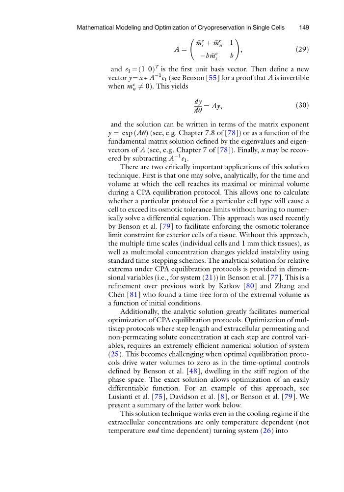
T is the first unit basis vector. Then define a new
vector y ¼ x + A
À1 e 1 (see Benson [55] for a proof that A is invertible
when m
e
n 6 ¼ 0). This yields
dy
dθ
¼ Ay,
ð30Þ
and the solution can be written in terms of the matrix exponent
y ¼ exp ðAθÞ (see, e.g. Chapter 7.8 of [78]) or as a function of the
fundamental matrix solution defined by the eigenvalues and eigenvectors of A (see, e.g. Chapter 7 of [78]). Finally, x may be recovered by subtracting A
À1 e 1 .
There are two critically important applications of this solution
technique. First is that one may solve, analytically, for the time and
volume at which the cell reaches its maximal or minimal volume
during a CPA equilibration protocol. This allows one to calculate
whether a particular protocol for a particular cell type will cause a
cell to exceed its osmotic tolerance limits without having to numerically solve a differential equation. This approach was used recently
by Benson et al. [79] to facilitate enforcing the osmotic tolerance
limit constraint for exterior cells of a tissue. Without this approach,
the multiple time scales (individual cells and 1 mm thick tissues), as
well as multimolal concentration changes yielded instability using
standard time-stepping schemes. The analytical solution for relative
extrema under CPA equilibration protocols is provided in dimensional variables (i.e., for system (21)) in Benson et al. [77]. This is a
refinement over previous work by Katkov [80] and Zhang and
Chen [81] who found a time-free form of the extremal volume as
a function of initial conditions.
Additionally, the analytic solution greatly facilitates numerical
optimization of CPA equilibration protocols. Optimization of multistep protocols where step length and extracellular permeating and
non-permeating solute concentration at each step are control variables, requires an extremely efficient numerical solution of system
(25). This becomes challenging when optimal equilibration protocols drive water volumes to zero as in the time-optimal controls
defined by Benson et al. [48], dwelling in the stiff region of the
phase space. The exact solution allows optimization of an easily
differentiable function. For an example of this approach, see
Lusianti et al. [75], Davidson et al. [8], or Benson et al. [79]. We
present a summary of the latter work below.
This solution technique works even in the cooling regime if the
extracellular concentrations are only temperature dependent (not
temperature and time dependent) turning system (26) into
Mathematical Modeling and Optimization of Cryopreservation in Single Cells
149
m
e
s þ
m
e
n
1
Àb
m
e
s
b
!
,
ð29Þ
and e 1 ¼ (1 0)
T is the first unit basis vector. Then define a new
vector y ¼ x + A
À1 e 1 (see Benson [55] for a proof that A is invertible
when m
e
n 6 ¼ 0). This yields
dy
dθ
¼ Ay,
ð30Þ
and the solution can be written in terms of the matrix exponent
y ¼ exp ðAθÞ (see, e.g. Chapter 7.8 of [78]) or as a function of the
fundamental matrix solution defined by the eigenvalues and eigenvectors of A (see, e.g. Chapter 7 of [78]). Finally, x may be recovered by subtracting A
À1 e 1 .
There are two critically important applications of this solution
technique. First is that one may solve, analytically, for the time and
volume at which the cell reaches its maximal or minimal volume
during a CPA equilibration protocol. This allows one to calculate
whether a particular protocol for a particular cell type will cause a
cell to exceed its osmotic tolerance limits without having to numerically solve a differential equation. This approach was used recently
by Benson et al. [79] to facilitate enforcing the osmotic tolerance
limit constraint for exterior cells of a tissue. Without this approach,
the multiple time scales (individual cells and 1 mm thick tissues), as
well as multimolal concentration changes yielded instability using
standard time-stepping schemes. The analytical solution for relative
extrema under CPA equilibration protocols is provided in dimensional variables (i.e., for system (21)) in Benson et al. [77]. This is a
refinement over previous work by Katkov [80] and Zhang and
Chen [81] who found a time-free form of the extremal volume as
a function of initial conditions.
Additionally, the analytic solution greatly facilitates numerical
optimization of CPA equilibration protocols. Optimization of multistep protocols where step length and extracellular permeating and
non-permeating solute concentration at each step are control variables, requires an extremely efficient numerical solution of system
(25). This becomes challenging when optimal equilibration protocols drive water volumes to zero as in the time-optimal controls
defined by Benson et al. [48], dwelling in the stiff region of the
phase space. The exact solution allows optimization of an easily
differentiable function. For an example of this approach, see
Lusianti et al. [75], Davidson et al. [8], or Benson et al. [79]. We
present a summary of the latter work below.
This solution technique works even in the cooling regime if the
extracellular concentrations are only temperature dependent (not
temperature and time dependent) turning system (26) into
Mathematical Modeling and Optimization of Cryopreservation in Single Cells
149