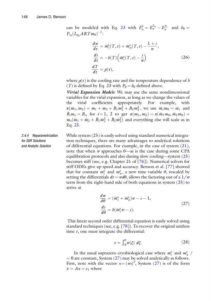
can be modeled with Eq. 23 with E
b
a ¼ E
L p
a À E
P s
a
and b 0 ¼
P s 0 ðL p 0 ART m 0 Þ
À1 :
dw
dτ
¼
m
e
s ðT , τÞ þ
m
e
n ðT , τÞ À
1 þ s
w
,
ds
dτ
¼ ÀbðT Þ
m
e
s ðT , τÞ À
s
w
dT
dτ
¼ gðτÞ,
ð26Þ
where g(τ) is the cooling rate and the temperature dependence of b
(T) is defined by Eq. 23 with P 0 ¼ b 0 defined above.
Virial Expansion Models: We may use the same nondimensional
variables for the virial expansion, as long as we change the values of
the virial coefficients appropriately. For example, with
πðm 1 , m 2 Þ ¼ m 1 þ m 2 þ B 1 m
2
1 þ B 2 m
2
2 , we use
m i m 0 ¼ m i and
B i m o ¼ B i , for i ¼ 1, 2 to get πðm 1 , m 2 Þ ¼ πð
m 1 m 0 ,
m 2 m 0 Þ ¼
m o ð
m 1 þ
m 2 þ
B 1
m
2
1 þ
B 2
m
2
2 Þ and everything else will scale as in
Eq. 25.
2.4.4 Reparametrization
for Stiff Solutions
and Analytic Solution
While system (25) is easily solved using standard numerical integration techniques, there are many advantages to analytical solutions
of differential equations. For example, in the case of system (21),
note that when w approaches 0—as is the case during some CPA
equilibration protocols and also during slow cooling—system (25)
becomes stiff (see, e.g. Chapter 21 of [76]). Numerical solvers for
stiff ODEs give up speed and accuracy. Benson et al. [77] showed
that for constant m
e
s and m
e
n , a new time variable θ, rescaled by
setting the differentials dτ ¼ wdθ, allows the factoring out of a 1/w
term from the right-hand side of both equations in system (25) to
arrive at
dw
dθ
¼ ð
m
e
s þ
m
e
n Þw À s À 1,
ds
dθ
¼ bð
m
e
s w À sÞ:
ð27Þ
This linear second order differential equation is easily solved using
standard techniques (see, e.g. [78]). To recover the original unitless
time τ, one must integrate the differential:
τ ¼
Ð θ
0
wðξÞ dξ:
ð28Þ
In the usual suprazero cryobiological case where m
e
s and m
e
n 6
¼ 0 are constant, System (27) may be solved analytically as follows.
First, note with the vector x ¼ (ws)
T
, System (27) is of the form
_
x ¼ Ax þ e 1 where
148
James D. Benson